How to Use Advanced Filter in Excel?
Understanding the Basics of Advanced Filter in Excel
Before we dive into the advanced functionalities of Excel’s Advanced Filter, let’s start with the basics. The primary purpose of this feature is to extract specific records from a data set based on user-defined criteria. Unlike the AutoFilter option, which is limited to filtering data within a single column, the Advanced Filter allows for complex filtering criteria across multiple columns simultaneously.
Advanced Filter Options
Excel’s Advanced Filter offers several additional options to enhance its functionality and flexibility. You can either filter your data in place or in a different place using this tool. So, let’s get familiarized with some of its features.
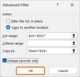
- Unique Records: By selecting the “Unique records only” checkbox in the Advanced Filter dialog box, you can filter out duplicate values, providing a streamlined view of your data.
- Copy to Another Location: Instead of specifying the output range within the same worksheet, you can choose to copy the filtered data to another location, such as a different worksheet or even a different workbook. This option allows you to keep your original data intact while working with filtered results.
- Using Formulas in Criteria Range: Advanced Filter enables the use of formulas within the criteria range, allowing you to perform calculations or use cell references to create dynamic filtering conditions.
- Combining Multiple Criteria: Excel’s Advanced Filter supports the use of multiple criteria within a column or across multiple columns. This capability facilitates advanced data analysis by allowing you to apply intricate filtering conditions.
How to Use Advanced Filter in Excel
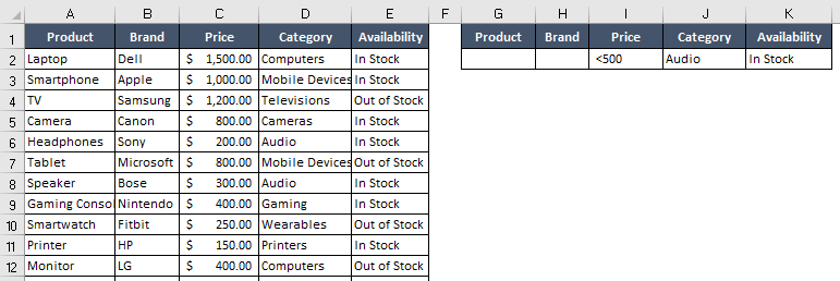
To explain the functionality of the Advanced Filter in Excel, I have created a dataset about some electronic items, their brand names, prices, and some other details. Here is a small glimpse of it.
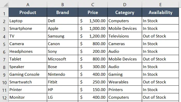
Now I will show you how I use the Advanced Filter on this dataset based on different situations and criteria.
Case 1: Unique Records Filtering By Advanced Filter in Excel
Sometimes the dataset contains duplicate data in the table, and you may need to filter out the unique values only. Although there are different methods to remove duplicates in Excel, using the advanced filter is one of the fastest.
Step-by-Step Guide
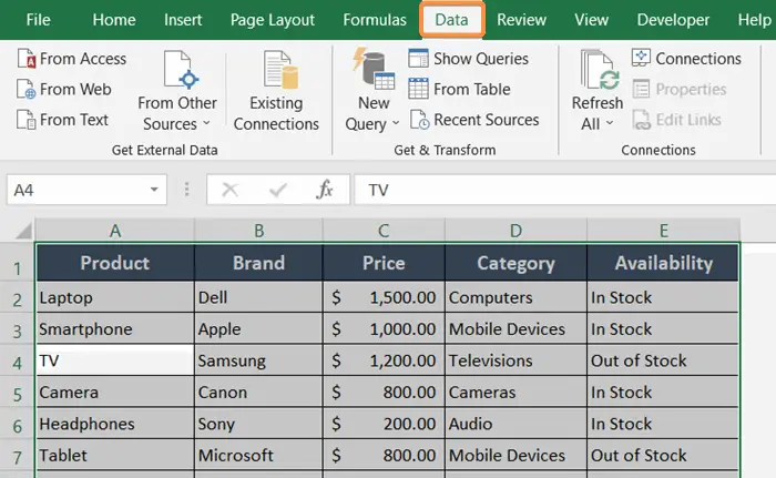
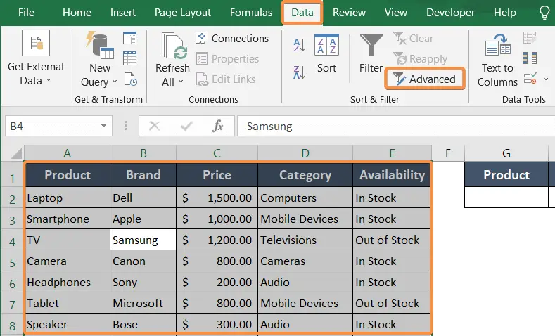
- Select the entire dataset, cell range A1:E27.
- Go to the Data tab.

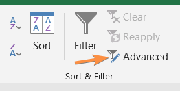
- Now click on the Advanced icon from the Sort & Filter group.
 The Advanced Filter dialog box will pop up on the screen.
 - Select Copy to another location from the Action section inside the dialog box.
- Review and check the List range.
The List range is supposed to refer to the cell range of the dataset. If not, then update it. - Keep the Criteria range empty.
- In the Copy to box, specify the cell address where you want the results to show.
- Next, checkmark the option Unique records only.
- Finally hit the OK button.

Final Result
This way you can create a table of unique results in a separate table.
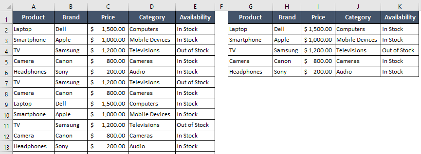
Otherwise, select Filter the list, in-place in the Advanced Filter dialog box to receive the results in the location of the dataset.
Case 2: Apply the AND Criteria in Advanced Filter in Excel
You can apply one or more criteria in the Advanced Filter and get the result meeting all the conditions according to that. When more than one criterion is applied, it is called the AND criteria.
Imagine that I want to find out about the Audio items that are now available under $500. Let me show you how I use the Advanced Filter to determine that.
Step-by-Step Guide
- First, copy the headers of the primary dataset and paste them somewhere in the worksheet.
I inserted it in cell G1. - Now insert the data filtering criteria in the new table.

- Now click on any cell of the main dataset and press CTRL+A.
This will select the whole data table. - Then go to the Data tab.
- Click on the Advanced icon from the Sort & Filter group.
 The Advanced Filter dialog box will pop up on the screen.
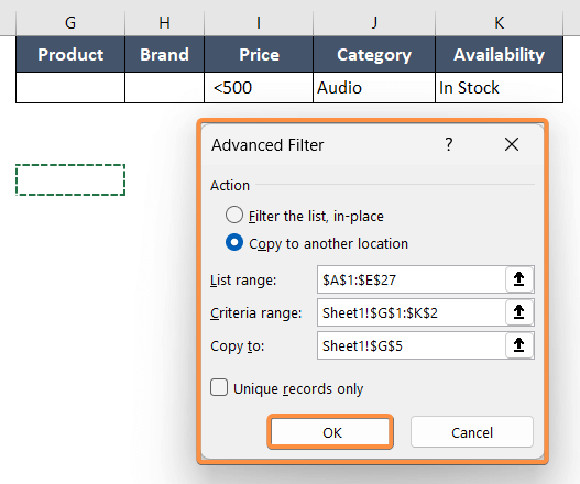
 - In the Action section, choose Copy to another location.
- Keep the List range unchanged.
The cell range of the dataset should be used as the List range. Also, update it if necessary. - In the Criteria range, mention the criteria range, G1:K2.
- Type the cell address where you want the result, cell G5 in the Copy to box.
- Hit OK.

Final Result
A new table in the same worksheet has been developed with data based on the criteria you mentioned.
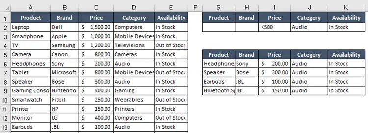
Case 3: Apply the BETWEEN Criteria in Advanced Filter in Excel
In some situations, you may need to locate numerical values that fall within a particular range. For example, I want to find Cameras of different brands that fall between the price range of $6,000 and $8,000.
Follow the directions given below to do that.
Step-by-Step Guide
- Copy the headers of the primary dataset and paste them anywhere in the worksheet.
- Add a second Price header after the first one that is currently present.
 Now insert the criteria this way:
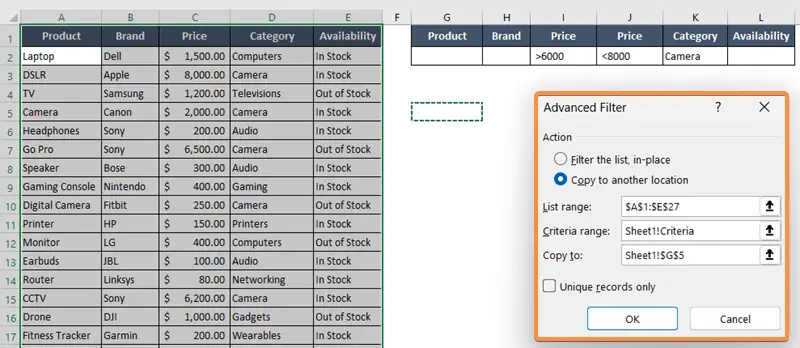
 I’m looking for cameras that are priced between $6,000 and $8,000.
- Next, select the dataset, A1:E27.
- Go to the Data tab.
- Select the Advanced command from the Sort & Filter group.
The Advanced Filter dialog box will appear. - Select Copy to another location in the Action section.
- Input the dataset cell range in the List range.
- In the Criteria range, mention the criteria range, G1:L2.
- In the Copy to box, type the cell address (cell G5) where you want the result.

- Click on the OK button.
Final Result
This way, you can insert range criteria in the Advanced Filter. You can see the result below:

Case 4: Apply the OR Criteria in Advanced Filter in Excel
By using the OR criteria in the Advanced Filter, you can add multiple sets of AND criteria. You may have noticed that while I used the AND criteria, the conditions were set in a single row. Now, as I apply the OR criteria, the conditions will be inserted in multiple rows.
Suppose I want to find the currently available Printers and Monitors on the market. In this situation, I will need to apply the OR criteria.
Step-by-Step Guide
- First, copy the headers of the primary dataset and paste them anywhere in the worksheet.
- Type the criteria under the headers.

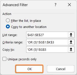
- Select the dataset, A1:E27.
- Go to the Data tab.
- Select the Advanced command from the Sort & Filter group.
The Advanced Filter dialog box will pop up. - Select Copy to another location in the Action section of the dialog box.
- Input the dataset cell range in the List range.
- In the Criteria range, mention the criteria range, G1:K3.
- In the Copy to box, type the cell address (cell G5) where you want the result.
- Press the OK button.

Final Result
Both conditions, filtering available Printers and Monitors, meet successfully using the OR criteria in Advanced Filter in Excel.
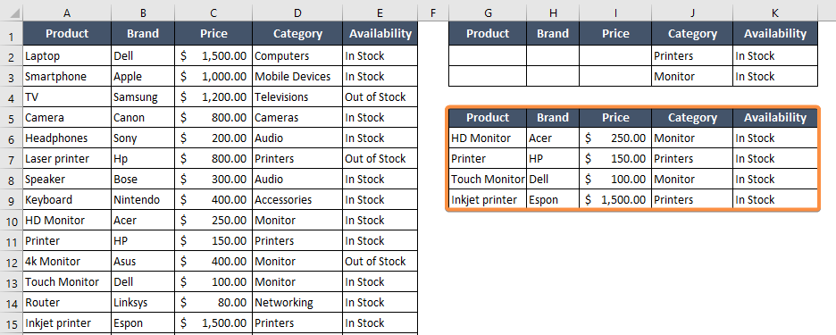
Case 5: Apply the Wildcard Criteria in Advanced Filter in Excel
Let me introduce you to three wildcard characters in the Advanced Filter that are going to save you a lot of time.
| Wildcard Character | Description |
|---|---|
| * (asterisk) | It represents any number of characters. |
| ? (question mark) | It represents a single character. |
| ~ (tilde) | It helps search for data containing an actual asterisk or question mark. |
1. Example of Wildcard Asterisk (*)
As I previously said, an asterisk (*) is used to represent any number of characters in the criteria range in Advanced Filter. It helps in the development of flexible searches that will accept different text patterns.
For example, here I used the criteria *TV to search any cell mentioning the word TV in the dataset.
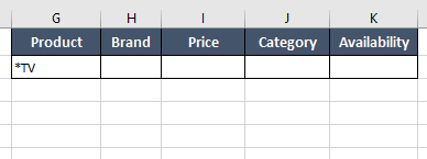
The search results found three words containing the word TV. Notice that the number of characters is different in each resultant cell.

2. Example of Wildcard Question Mark (?)
The question mark (?) is another wildcard character used in the Advanced Filter of Excel. The question mark (?) has two functionalities. It is known for representing a single character within a text string and it can also be used as an asterisk (*).
Here I have S? in the criteria field.
 As I applied the Advanced Filter, the result showed all the cells that have the starting letter S.
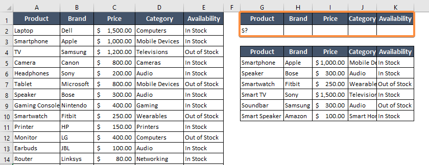
When defining your filtering criteria, you can use the question mark to represent any single character. For example, if you want to filter a list of words and find all five-letter words where the third letter is a, you can use the criteria ??a??. This will match any word with five letters where the third letter is a and the other letters can be any character.
3. Example of Wildcard Tilde (~)
The tilde (~) is a special character known as an escape character in the Advanced Filter in Excel. It is used to treat wildcard characters (asterisks or question marks) as literal characters.
For example, in the dataset, I have some cells containing the asterisk (*) in the middle of the words. So, in the criteria table, I inserted *~* as the criteria.
 The result is in the following image:
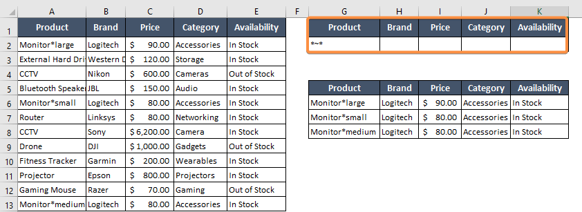
Here, when I want to filter text that starts with a series of letters, I use an asterisk (*) at the beginning of my criteria. In the middle of the text, there is an actual asterisk (*) that I want Excel to treat as a literal character rather than a wildcard. To achieve this, I added a tilde (~) before the asterisk (*) in my criteria. This ensures that Excel understands it as a literal asterisk and doesn’t confuse it with a wildcard character. After the wildcard, there is another series of letters. So I added another asterisk (*) at the end.
Conclusion
I hope you get a clear concept of the different uses of the Advanced Filter. Follow the step-by-step guidelines provided in this article to apply the Advanced Filter in the Excel worksheets. I hope you find this blog helpful. Let me know in the comment section if you need clarification about this topic. Have a good day!
Excel Glossary | Autosum | Fill Handle | Conditional Formatting | Merge & Center | Wrap Text | Flash Fill | Find & Replace | Freeze Panes | Format Painter | Format Cells | Sort & Filter | Text to Columns | Go To Special | Calculation Options | Name Manager | Excel Table | Slicer | Power Query | Add-ins
 The Advanced Filter dialog box will pop up on the screen.
 The Advanced Filter dialog box will pop up on the screen.
 Now insert the criteria this way:
 I’m looking for cameras that are priced between $6,000 and $8,000.