4+ Ways to Find Duplicates in a Column and Delete Rows in Excel

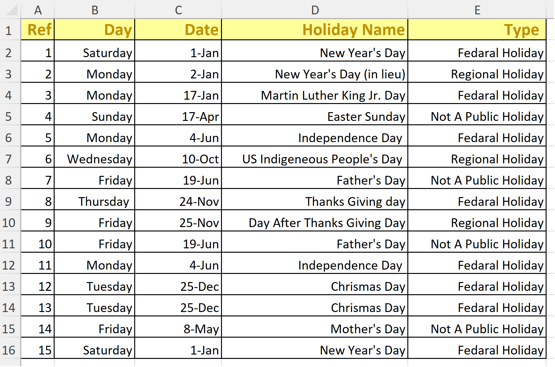
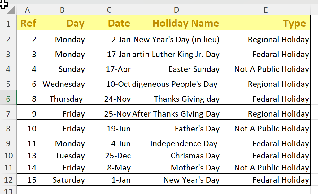
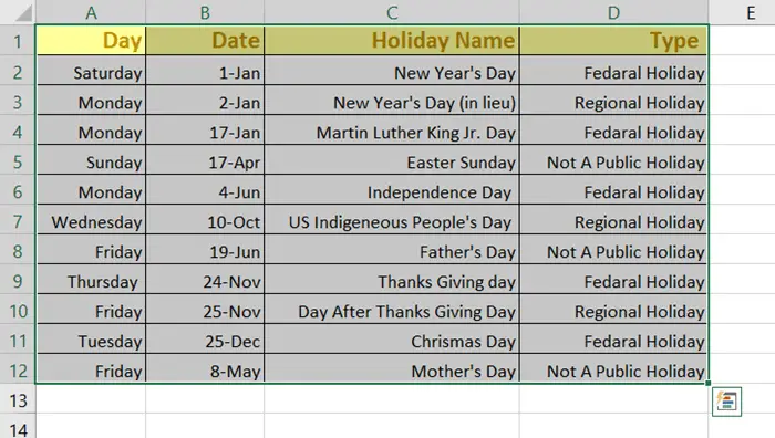
Duplicate data can be a real pain. It often sneaks up on you when you merge different datasets. In a small table you might be able to spot duplicates manually, but the problem gets bigger as your data grows. To tackle this issue, let’s look at 4 ways to find duplicate values in columns and then delete rows in Excel.

The dataset I have used throughout this article (download at the button below the image⬇️) contains columns with details of different holidays in the USA:

Feel free to download our example workbook, and follow along:

Find Duplicates in Column and Delete Rows in Excel.xlsx

Table of Contents

Method 1 (easiest): Filter and Remove Duplicate Values in Excel with the Remove Duplicates Command

The simplest way to remove duplicates in a dataset is by using the built-in Remove Duplicates command. It identifies duplicates and deletes them, so that only unique values remain. To do that, follow the steps below:

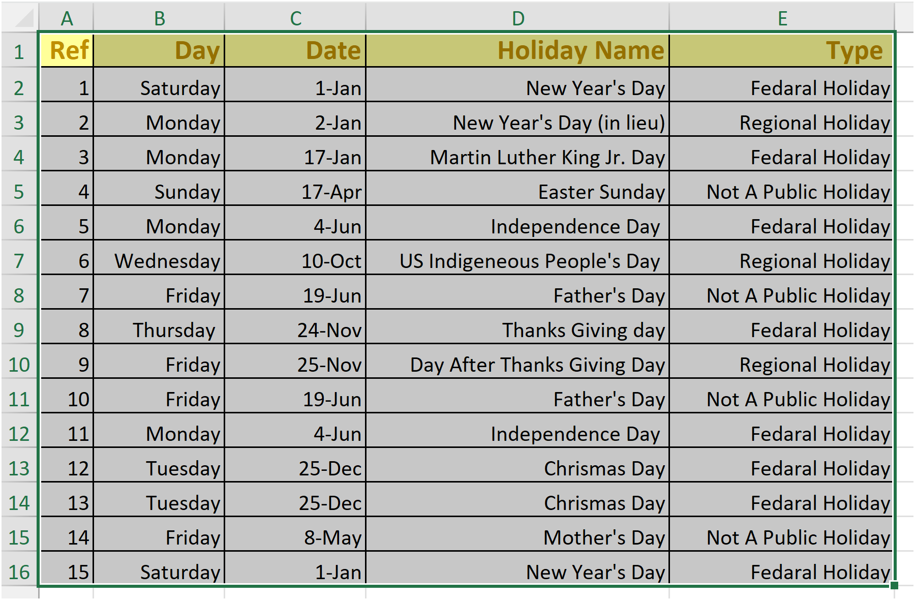
Step 1: Select the entire data table (click anywhere in the dataset and press CTRL+A).
Find Duplicates in Columns and Delete Row

Step 2: On the Data ribbon, under the Data Tools group, click on the Remove Duplicates command. Or use keyboard shortcut Alt, A, M.

You will see the Remove Duplicates dialog box will pop up.

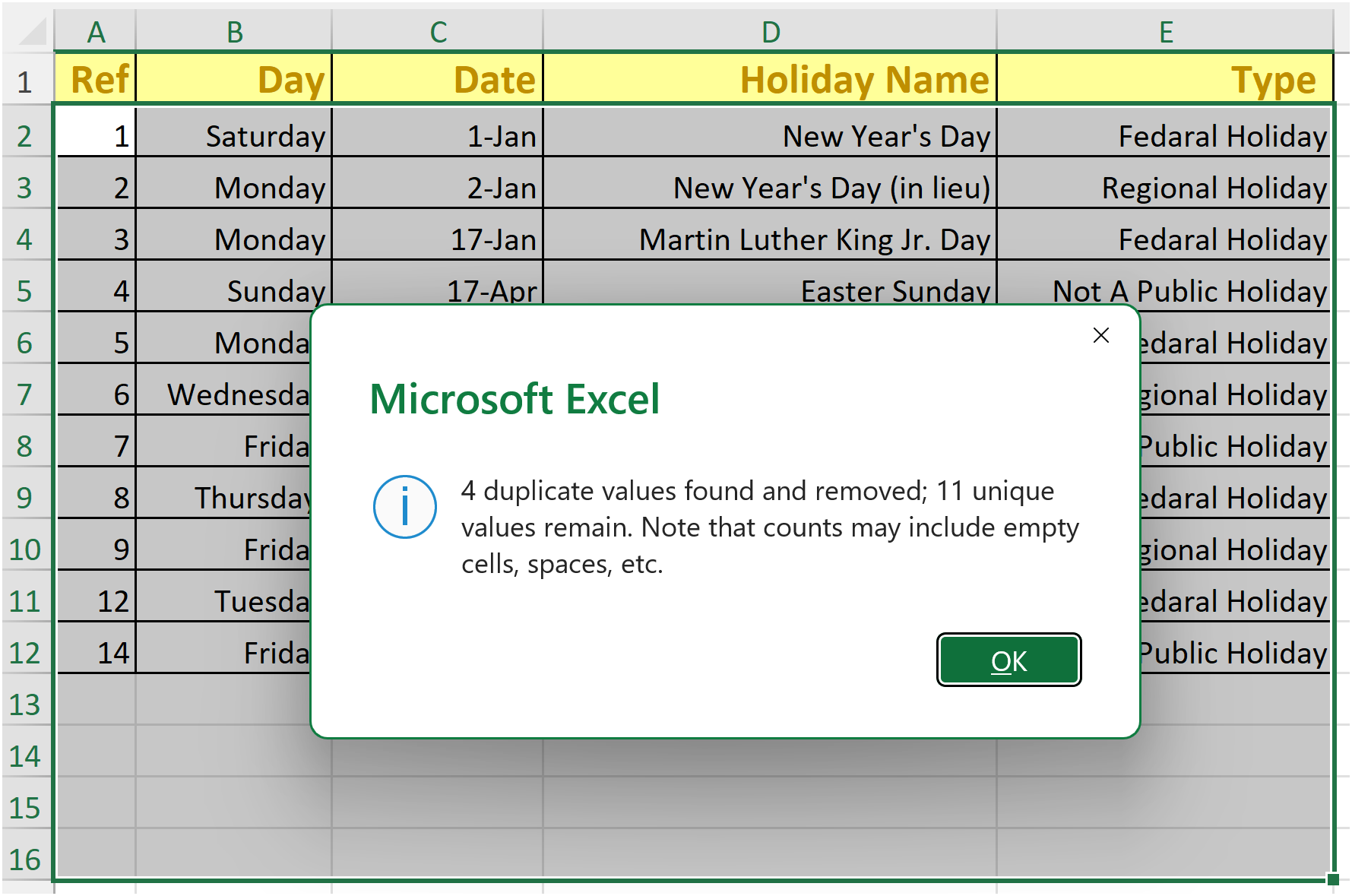
Step 3: In this dialog box, tick all the columns that need to be checked for duplicates, before the row is considered a duplicate for deletion. E.g. in our example below, the first column is just a counter and can be ignored, but columns B to E should all be checked for duplicates. If all four these columns match, then the row is considered a duplicate and will be deleted.

Also, check that the My data has headers checkbox is selected, and click OK.

After clicking OK, you will see a dialog box that shows the number of duplicates found (i.e. the number of rows that have been deleted), as well as the number of unique items remaining:

Method 2: Use Conditional Formatting to Find Duplicates in Columns, then Delete Rows

You can also use Conditional Formatting to detect duplicates in columns, and then delete the duplicate rows. Excel has a built in function where it automatically highlights duplicate cells in a column.

But be careful, in order for Conditional Formatting to pick up a real duplicate row, we need to create an extra column that concatenates all of the values together, and then we only assess this new column for duplicates.

I can hear you asking, “Why can’t we just apply conditional formatting to the whole table and then look for rows that are completely highlighted?” The reason is simple… This approach might lead to false positives, and as a result unique rows can be deleted in error.

Look at this example – The table below lists the pupils from a few different schools, who scored 100% in a subject: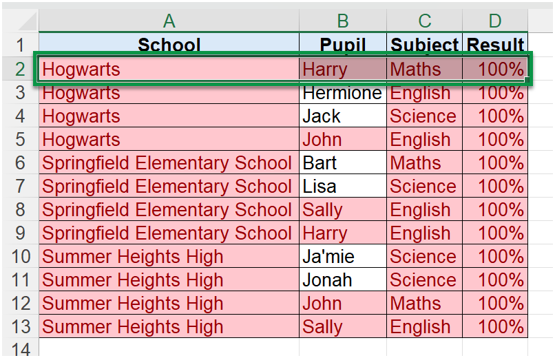 False duplicates in a range in excel

In this image it looks like there are a number of rows that are duplicates, e.g. in row 2: Harry from Hogwarts, who scored 100% in Maths. We can see that all four columns are highlighted for this item, so this row must be a duplicate…right?

Nope! If we look closely, we can see that NONE of the records are duplicated. The only other Harry is on row 9, but this Harry is from Springfield Elementary, and scored 100% in English. So yes, every item is duplicated somewhere, but there are no rows where the entire row is a duplicate of another row. If we deleted one of these rows then we would have accidentally deleted a unique record.

To prevent this from happening, we need to create a helper column that concatenates (glues together) the values from ALL of the other columns, and then we assess this new column for duplicates.

Here are the steps:

Step 1: First we need to create our helper column. In cell E2, enter the following formula:

=CONCATENATE(B2, C2, D2, E2)

Or, if you are using a newer Excel version (after Office 2016):

=CONCAT(B2:E2)

Step 2: Double click the little fill handle in cell F2, to copy the formula all the way down to cell F16.

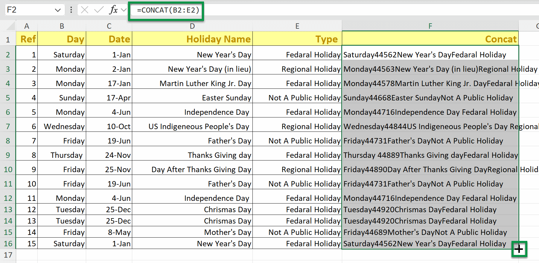
We can now go ahead and check the concatenated column (col F) for duplicates, using Conditional Formatting.

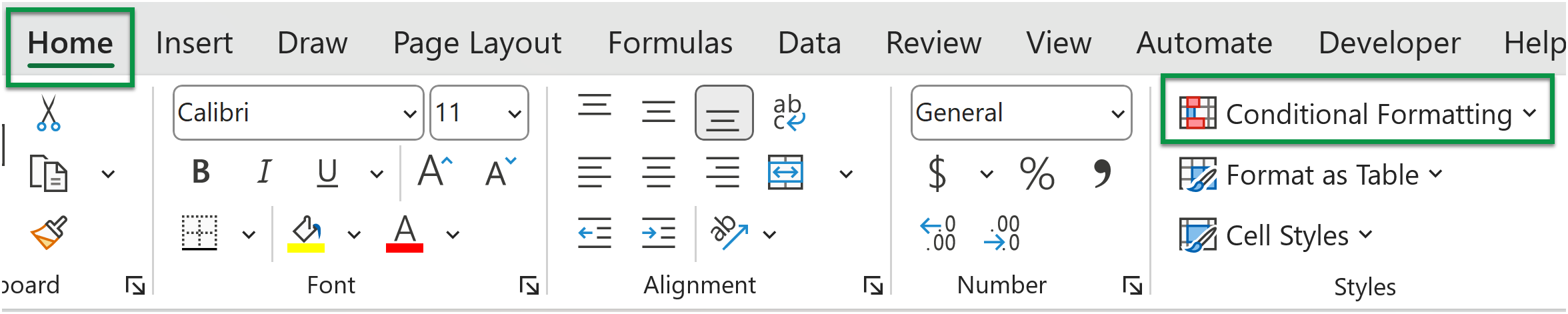
Step 3: Make sure the concatenated column is still selected. On the Home ribbon, under the Styles group, click Conditional Formatting…

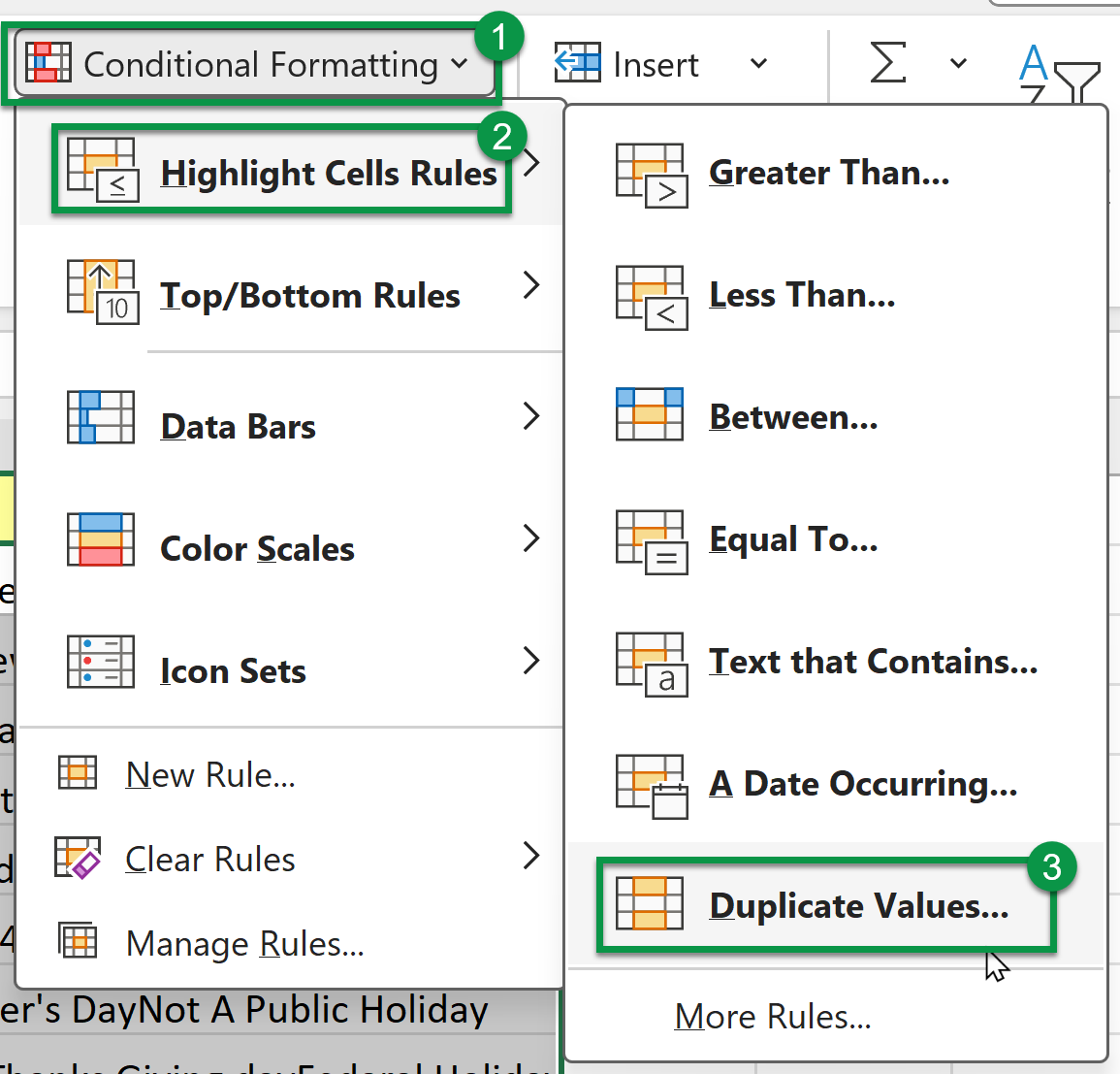
…then Highlight Cell Rules… then Duplicate Values:

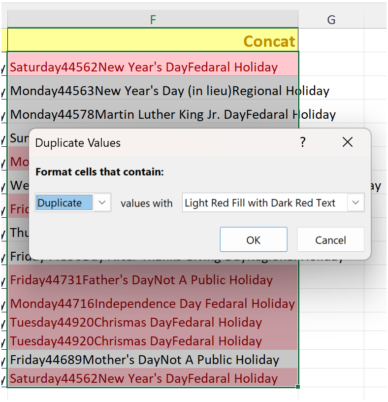
Step 4: Here we can make changes to how duplicates will look, or just click OK to highlight all the duplicates in Light Red Fill with Dark Red Text:

We can now add a Filter to the column, to only show the duplicate rows in the table.

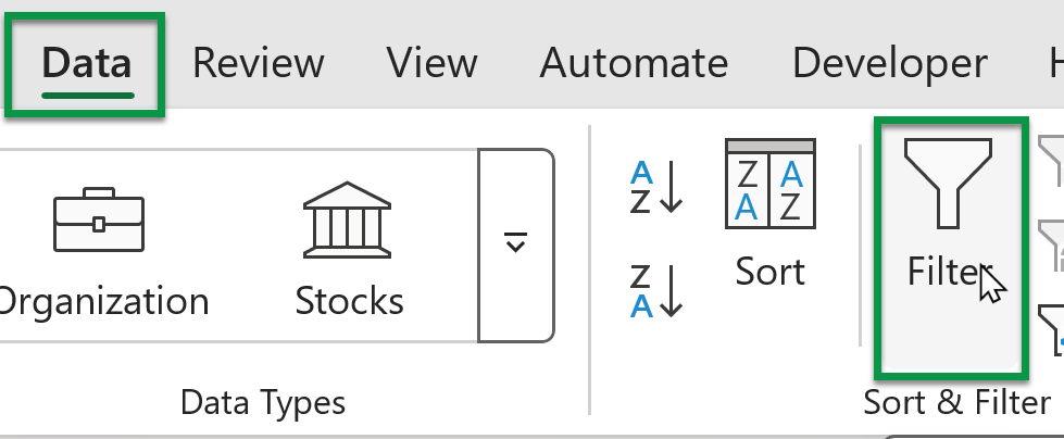
Step 5: Select the concatenated column F (including the heading), and on the Data ribbon, click Filter:

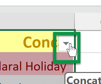
This adds a little drop-down twisty to the right-hand side of the heading cell:

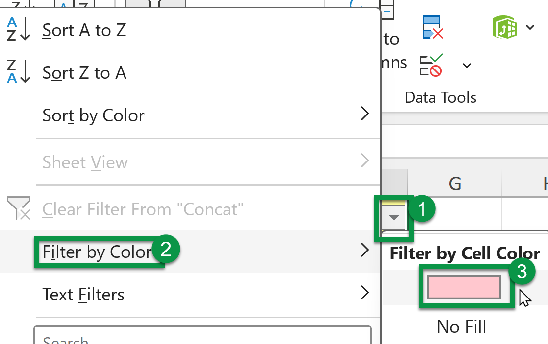
Step 6: Filter the concatenated column by clicking the twisty in that column, and selecting Filter by Color, then picking the appropriate text colour or cell background to show the duplicates:

Now we decide what we want to delete…

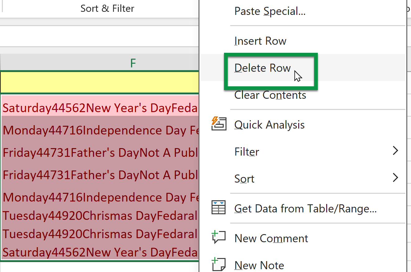
Step 7(a): Maybe we want to get rid of all items that are/have duplicates. E.g. if there are three items, “Apple”, “Banana” and “Banana”, we want to delete both instances of “Banana” but keep “Apple” as it had no duplicates. Here, both instances of “Banana” would already be highlighted, so we can just select and delete them both. So in this example, we select all of the pink cells, right click somewhere in the selected range and click Delete Row:

Step 7(b): Alternatively, you may want to delete only the duplicates and leave one unique copy of each item. I.e. keep the first instance but delete all other instances of that item. To do this, we make sure only one item is selected, then right click, and select Delete Row. After deleting a row, if there is only one copy of that item remaining, it will no longer be highlighted:

Keep doing this, until there are no duplicates left and only unique items remaining.

PRO TIP: A quick way to do this is by immediately selecting the next duplicate, then pressing F4 (redo last action). You can keep moving to other duplicates and pressing F4, until there are no duplicates left. But make sure you don’t perform any other steps while you are deleting with F4, as F4 repeats your last action. If you did anything else (even saving the document), then you will need to delete another row first, before pressing F4 again.
F4 (redo last action) can be super powerful when it comes to saving time, but you have to be careful when using it, so you don’t accidentally redo the wrong action!

Step 8: We can now clear the Filter, and even delete the helper column, as we are done dealing with duplicates:

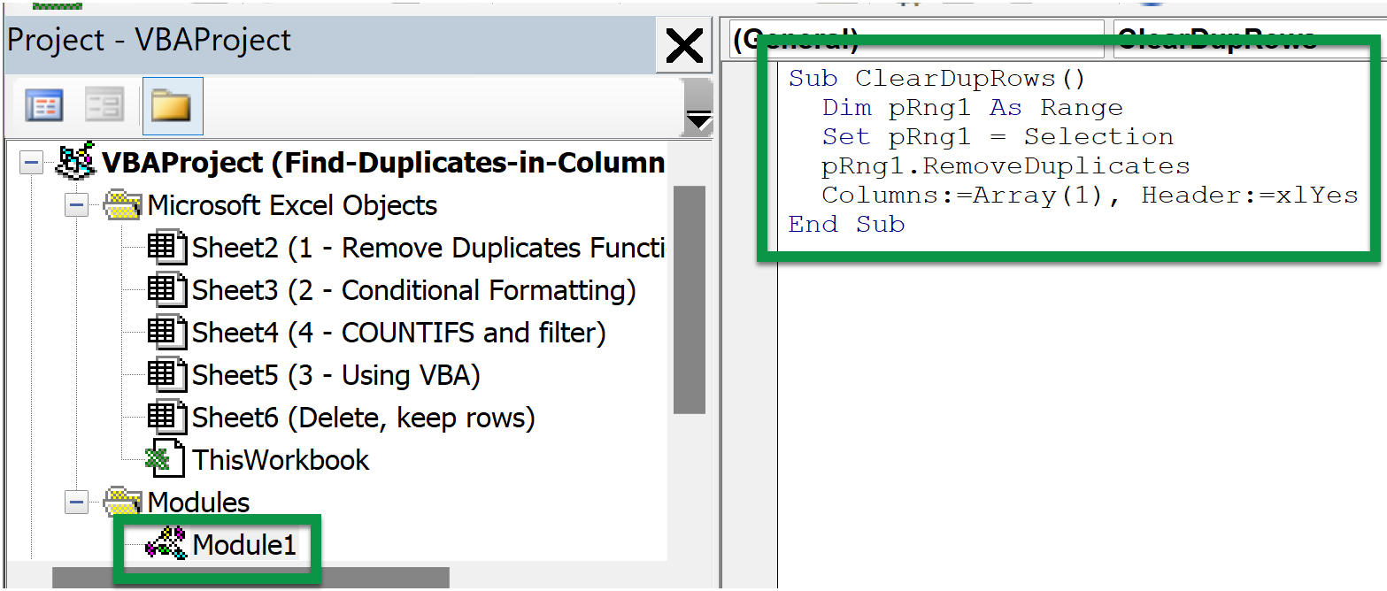
Method 3: Find Duplicates in Columns and Delete Rows in Excel Using VBA Macros

Apply VBA Macros to find duplicates in columns and delete rows in Excel. So, here are the steps below:

Select the entire data table.
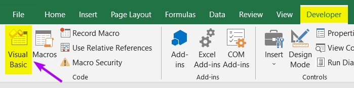
Click on the Developer tab from the ribbon. (No Developer tab? Learn how to add it to the ribbon).
Click on the Visual Basic command, under the Code group. Or press keyboard shortcut Alt-F11.
The Visual Basic Editor will open.
On the Insert menu, select Module:

Insert this Macro in the blank area on the right-hand side of the Visual Basic Editor.

Sub ClearDupRows() 
Dim pRng1 As Range 
Set pRng1 = Selection
pRng1.RemoveDuplicates Columns:=Array(1), Header:=xlYes 
End Sub

Insert VBA to remove duplicates

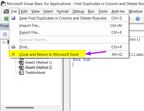
From the top-left corner, click on the File drop-down list.
Hit the Close and Return to Microsoft Excel option.
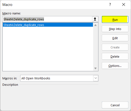
Again select the Developer tab and select the Macros command under the Code group.
Or, press ALT+F8 to open the Macro dialog box.
In the Macro dialog box, select the newly created macro, then click the Run button.

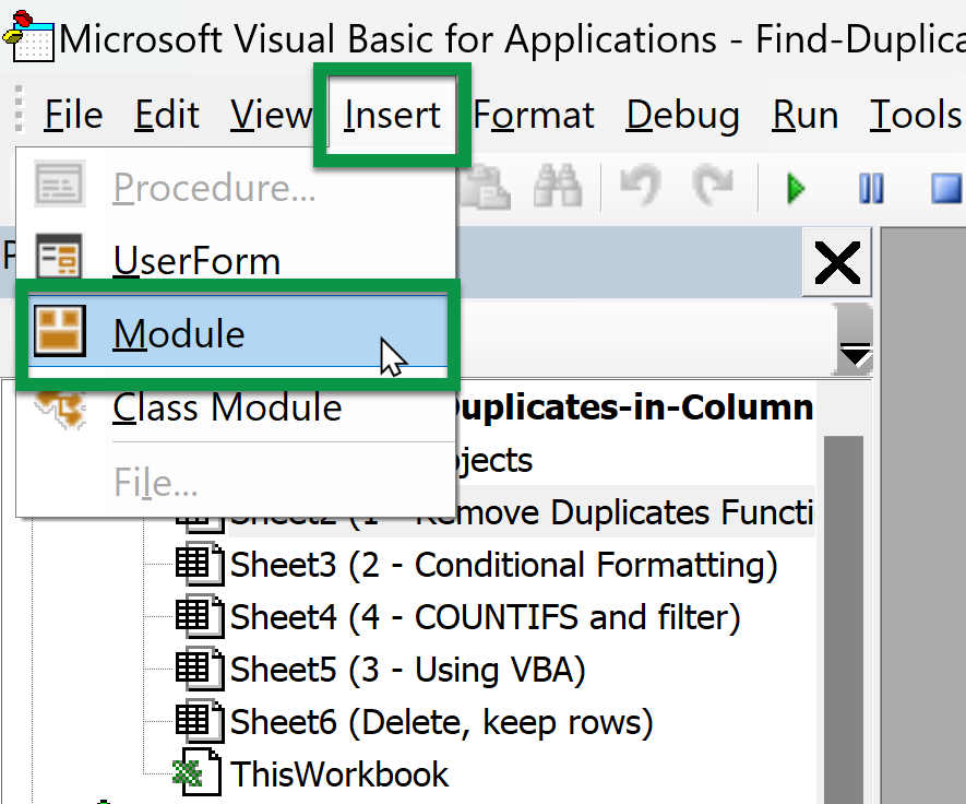
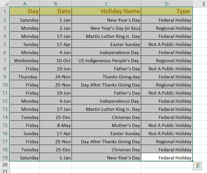
Now, the duplicated values are gone from the list.

Method 4: Find Duplicates in Columns and Delete Rows with COUNTIFS Function & FILTER Command

Use the COUNTIFS function to detect similar values in Excel.

Syntax

COUNTIFS(criteria_range1, criteria1,..)

Formula

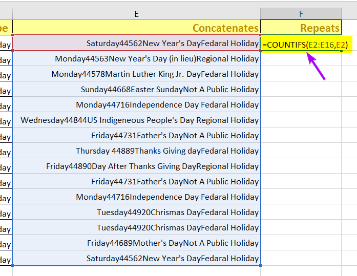
=COUNTIFS(E2:E16,E2)

Formula Explanation

The formula counts the number of occurrences of the value in cell E2 within the range E2:E16.

Formula

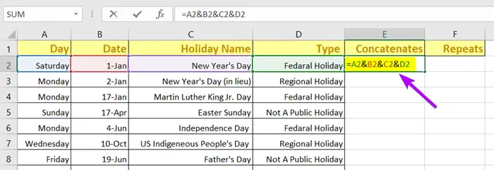
=A2&B2&C2&amp;D2

Formula Explanation

This formula will link up the top cells of each column together.

To find duplicates in columns and delete rows with COUNTIFS function, follow these steps below:

Create two new columns beside the data table (Column E & F).
Type this formula inside cell E2: =A2&B2&C2&D2
Press ENTER to join the cells together.
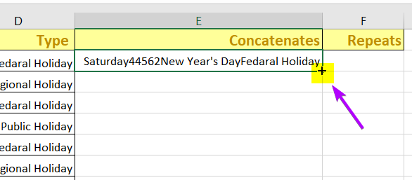
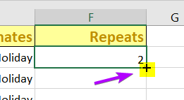
Double-click on the Fill Handle.
This will copy the formula toward the entire column.
Copy this formula and paste it into cell F2: =COUNTIFS(E2:E16,E2)
Press ENTER.
Double-click on the Fill Handle.
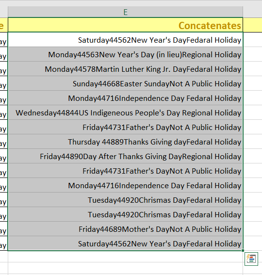
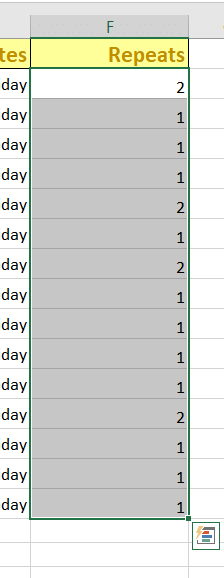
The total count of repetitions will show up in column F.I will filter the duplicates now.
Select the Data tab from the ribbon.
Under the Sort & Filter group, click on the Filter command.
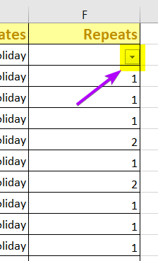
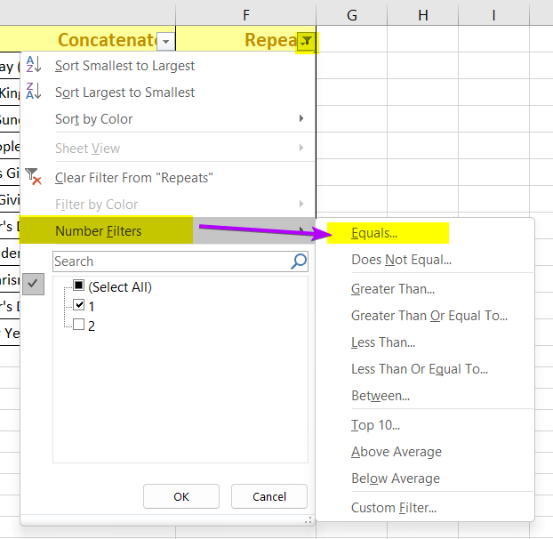
Right-click on the filter dropdown icon.
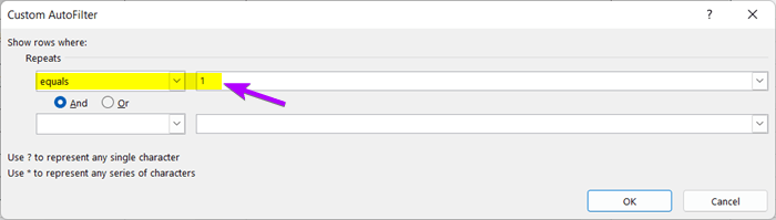
Select Number Filters > Equals command.
In Custom AutoFilter dialog box, select Equals and type ‘1’ in the empty box beside Equals under the Repeats dropdown. Then, hit OK.
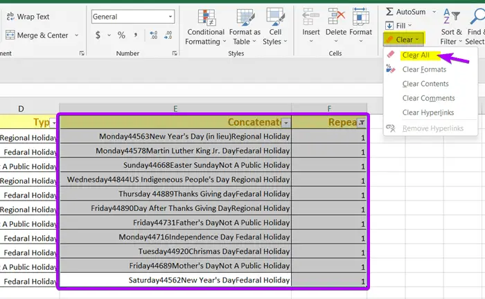
Now, select column E and column F.
Click on the Home tab > Editing group > Clear drop-down menu > Clear All command.

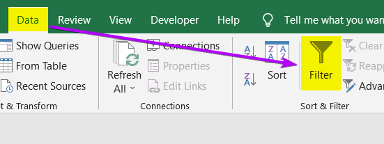
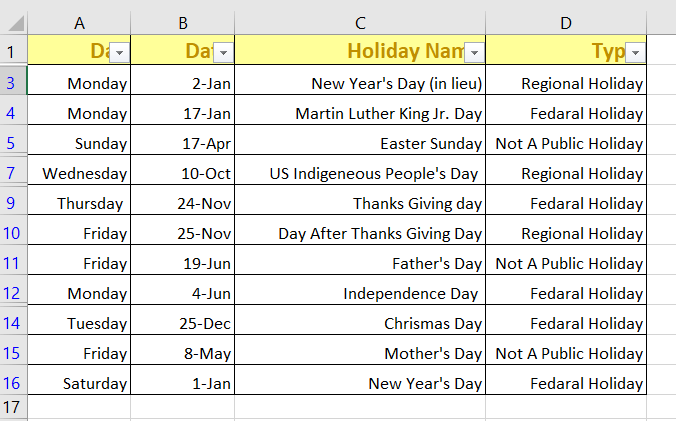
I have removed column E and column F from my dataset to keep it neat and clean.

Conclusion

We looked at 4 ways to find duplicates in multiple columns and then delete the duplicate rows. I hope you’ve found your required solution from this blog. Tell us how you like the solutions in the comment section!

Frequently Asked Questions

What is the easiest way to remove duplicates in Excel?

The easiest way to remove duplicates in Excel is by clicking somewhere in your dataset, then pressing the keyboard shortcut Alt, A, M.

This will bring up the Remove Duplicates dialog. Here, select all the columns that contain duplicates (i.e. that we want to be unique), and press OK. All duplicate rows have now been deleted.

What is the formula for finding duplicates in Excel?

The formula for finding duplicates in Excel is =COUNTIF(A:A, A2)>1

Here A:A is the column containing the data, and A2 is the first cell in that column (we’re assuming A1 is the column heading). This formula checks if the value in a cell appears more than once in the specified column. So for all duplicates, this formula will bring back a value of 2 or higher.

We can now filter to show only the cells that show TRUE, and delete those rows.

How do I delete non duplicates in Excel?

To delete non-duplicates in Excel, create a helper column with the formula =COUNTIF(A:A, A2)=1
Filter to show only rows that have TRUE in the helper column (i.e. the non-duplicate rows).
Delete all the non-duplicate rows.

Why should we remove duplicates?

Removing duplicates in data is essential to enhance accuracy and streamline analysis by eliminating redundant information, ensuring data integrity, and preventing errors in statistical calculations or decision-making processes.

Rate this post