How to Use XMATCH Function in Excel [4 Examples]

In the realm of Excel functions, XMATCH stands out as a powerful tool for searching and matching data within a range or array. Whether you’re a seasoned Excel user or just starting to explore its capabilities, understanding the XMATCH function can significantly enhance your data manipulation skills. In this guide, we’ll delve into the intricacies of the Excel XMATCH function, exploring its syntax, arguments, and output, and providing practical examples to illustrate its usage.

Table of Contents

What Does the Excel XMATCH Function Do?

The XMATCH function in Excel is designed to search for a specified value within a range or an array and return the relative position of that value. It offers more flexibility and features compared to its predecessor, the MATCH function, making it a valuable asset for various data analysis tasks.

What is the Syntax of the Excel XMATCH Function?

The syntax of the XMATCH function is as follows:

=XMATCH(lookup_value, lookup_array, [match_mode], [search_mode])

What are the Arguments of the Excel XMATCH Function?

lookup_value: The value you want to search for within the lookup_array.
lookup_array: The range or array where the lookup_value will be searched.
[match_mode]: (Optional) Specifies the type of match to be performed. It can take three values: 0 for an exact match, -1 for an exact match or the next smaller item, and 1 for an exact match or the next larger item. The default is 0.

[search_mode]: (Optional) Determines the search method to be used. It can take three values: 1 for searching from top to bottom, -1 for searching from bottom to top, and 2 for searching in binary mode (lookup_array must be sorted in ascending order). The default is 1.

What is the Output of the Excel XMATCH Function?

The XMATCH function returns the relative position of the lookup_value within the lookup_array. If Excel does not find the value, it returns the #N/A error.

4 Examples of Using the XMATCH Function in Excel:

Now, let’s explore some practical examples to understand how the XMATCH function works in real-world scenarios.

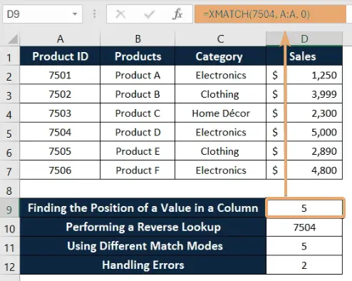
Example 1: Finding the Position of a Value in a Column

Suppose we have a list of students’ scores in column A, and we want to find the position of a specific product ID, say 7504.

=XMATCH(7504, A:A, 0)

This formula will return the position of 7504 within column A.

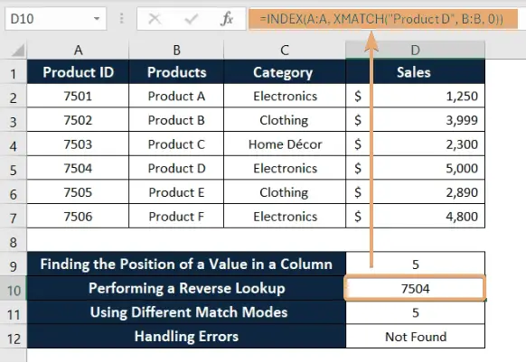
Example 2: Performing a Reverse Lookup

In this example, we have a list of product IDs in column A and their corresponding names in column B. We want to find the price of a specific product, say “Product D”.

=INDEX(A:A, XMATCH("Product D", B:B, 0))

This formula uses the XMATCH function to find the position of “Product D” in column B and then retrieves the price from column A using the INDEX function.

Example 3: Using Different Match Modes

Suppose we have a sorted list of product prices in column D, and we want to find the position of the price to $5000.

=XMATCH(5000, D:D, -1, 1)

It will output the position of the nearest smaller value. If 5000 is smaller than all values in column D, it will return an error.

Example 4: Handling Errors

If Excel does not find the lookup_value in the lookup_array, the XMATCH function returns an #N/A error. We can use the IFERROR function to handle this scenario gracefully.

=IFERROR(XMATCH("Grocery", C:C, 0), "Not Found")

If Excel does not find the value “Grocery” in column C, the formula will return “Not Found.”

Things to Remember

Make sure to properly sort the lookup_array, particularly when employing binary search mode.
Use error handling techniques like IFERROR to deal with potential errors.
Experiment with different match modes to achieve the desired results.

Conclusion

Mastering the XMATCH function in Excel can significantly boost your productivity and efficiency when working with large datasets. By understanding its syntax, arguments, and various applications through practical examples, you can leverage its power to perform complex data lookups and manipulations with ease.

Frequently Asked Questions

What is the difference between XMATCH and MATCH functions?

The XMATCH function offers additional features such as support for reverse lookup and more flexible match modes compared to the MATCH function.

Can XMATCH handle approximate matches?

Yes, XMATCH can handle both exact and approximate matches using different match modes.

Is it necessary to sort the lookup_array for XMATCH to work?

It depends on the match mode it utilizes. For binary search mode (search_mode = 2), the lookup_array must be sorted in ascending order.

How does the XMATCH function handle errors?

If the XMATCH function cannot find the lookup value within the lookup array, it generates the #N/A error. To handle this scenario gracefully, users can use error-handling techniques such as the IFERROR function to display custom messages or perform alternative actions.

Is it necessary to sort the lookup array for XMATCH to work?

The necessity to sort the lookup array depends on the match mode being used. For binary search mode (search_mode = 2), the lookup array must be sorted in ascending order. However, for other match modes, sorting the array is not mandatory but may still be beneficial for better performance.

Can XMATCH be used for performing reverse lookups?

Yes, one of the key features of the XMATCH function is its ability to perform reverse lookups, meaning it can search for a value in one column and return a corresponding value from another column. This capability makes it particularly useful for data analysis and referencing tasks.

Rate this post