How to Sort Multiple Columns in Excel (4 Ways)

Sorting data in Excel is quite a common task that we need to do. Sorting can be done based on several criteria. You can sort either single or multiple columns as well as rows in Excel. In this article, you will learn 4 ways to sort multiple columns in Excel with ease.

Sorting Multiple Columns in Excel.xlsx

Table of Contents

Sort Multiple Columns in Excel with Keyboard Shortcut

To sort multiple columns in Excel, follow these steps below:

Select the whole data table.

Press CTRL + SHIFT + L to apply Filter.
Now click on the drop-down icon of the column headers and sort them.

Sort Multiple Columns in Excel without Mixing Data by Custom Sort Command

The quickest and easiest way to sort multiple columns in Excel is to use the Custom Sort command. Now, follow the steps below to learn the whole process:

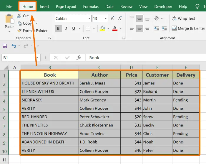
Select the entire table first.
Then, go to the Home tab.

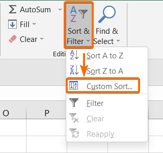
From the Edit group, click Sort & Filter.
From the drop-down list, choose the Custom Sort command.
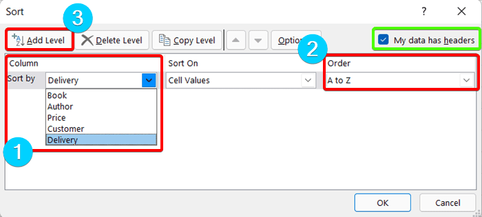
Then the Sort dialog box will appear. From the Sort by drop-down (under the Column section), select the first column name.
For this instance, I’m picking the Book column.

After that choose your preferred order from the Order drop-down list. I’m choosing A to Z here.
Click on the My data has headers command (right above the Order section) if your data table has a header.
To apply the sorting criteria to another column, click on the Add Level command.

Pick another column name from the Then by drop-down and change its order from the Order drop-down.
You can customize your data list from the Custom List command inside the Order drop-down.
Finally hit the OK button to apply changes.

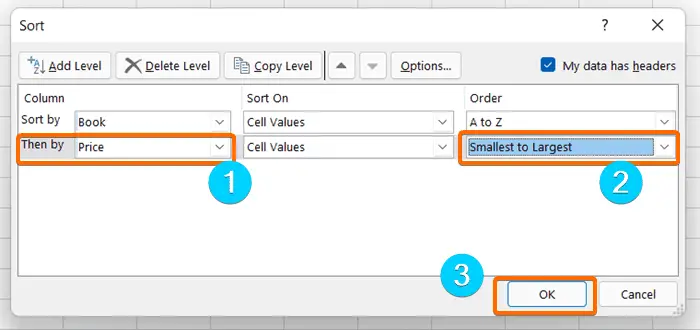
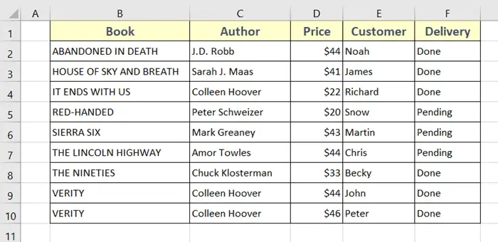
After completing all the steps above, you will see your data table is sorted as per your customization like the image below:

Sort Multiple Columns in Excel Utilizing Sort Command

There is another technique that you can use that will lead you to the same Sort dialog box to sort multiple columns. To do that, follow these steps below:

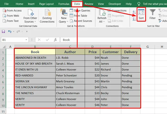
Select the whole table.

Then click the Data tab.
Click on the Sort command from the Sort & Filter group.
The Sort dialog box will appear then.
Before bringing any changes, make sure that the My data has headers command is checked.

Then, click on the Sort by drop-down from the Column group and select the first column name you want to sort.
In this case, I am choosing the Delivery column.
Next, change the order from the Order column. I am choosing alphabetically A to Z order here.
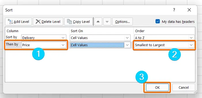
Click on Add Level if you want to sort another column.

Choose another column to sort from the Then by drop-down.
Then, change the Order of it. Hit OK to save the changes.

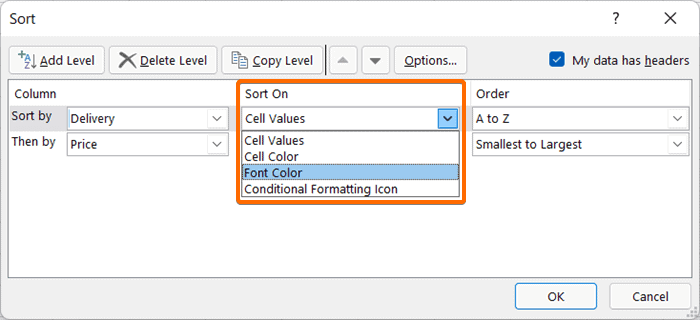
Note that, apart from sorting by the Cell values, you can also sort your table by using the Sort on command. Such as, by changing its Cell color, Font color, etc. (if your table has multiple colors in it).

Sort Multiple Columns in Excel Using the Filter Command

To sort multiple columns in Excel with the Filter command, here are the steps below:

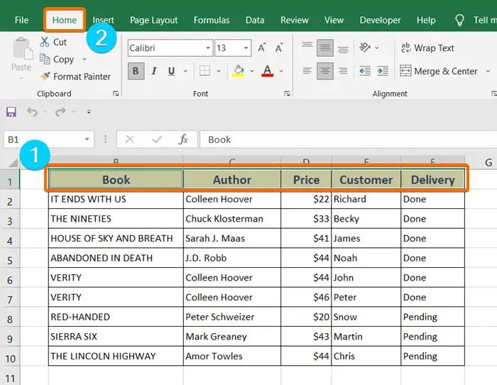
Select the full row of the headers of the table.
Now, click on the Home tab.
Hit click on the Sort & Filter drop-down located in the Editing group of commands and hit Filter.
You will see small arrows of the Filter command will show up beside each header.

Then, select the first header from the column list.
I picked the price column and sorted it by the Largest to the Smallest arrangement.

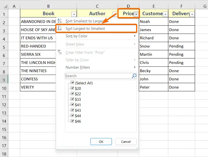
After sorting the price column, the column will appear with an arrangement like the image below:

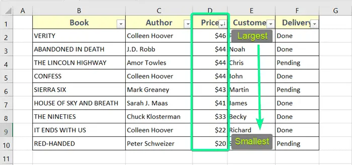
Then, again choose the next header and sort it as you like. By using this technique, you can sort the data from multiple columns.

How to Sort in Excel by Date (3 Ways)

Sort Multiple Columns in Excel Applying Conditional Formatting

Another technique for sorting multiple columns is using Conditional Formatting where the columns will be highlighted with different colors or symbols. Don’t worry, the orders of your data will not change. The colors of the data will only point out different values of the data.

Note that, this command is only for numerical sorting arrangements (such as price, size, salary, date, etc.).

So, apply Conditional Formatting in Excel, go through these steps below:

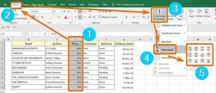
Select the first entire column (of course with numerical values) from the table.

Then, hit the Home tab from the Excel ribbon.
Click on the Conditional Formatting drop-down, where you will find the Color Scales drop-down.
Now, choose any of the color scales you like.
I have selected the White-Red color scale for the Price column. The white color denotes the lowest price on the list, and the red color means the highest price.

Next, choose another column to sort. For example, I have selected the Delivery Date column as it contains numbers.
Then, again select the Color Scales command from the Conditional Formatting drop-down.
This column doesn’t need to be of the same color scale as the previous column.
Pick any of the color styles you want.
I have selected the Green-Yellow color scale where the yellow cells indicate the older dates and the deep green cells indicate the latest dates.

The resulting table looks like the image below:

How to Sort Rows in Excel

Most of the time when we sort data in Microsoft Excel, we sort the data by columns. But you can sort your data by rows also, just like you sort the columns. Sometimes you will need to sort the spreadsheet with rows in some cases.

Follow the steps below to sort data in rows in an Excel sheet:

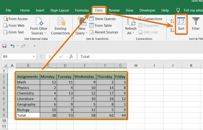
Select the entire table.
Then, click the Data tab from the ribbon.

Next, select the Sort command from the Sort & Filter group.
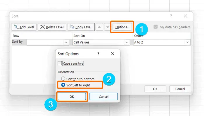
You will see the Sort dialog box will pop up.
Click on the Options button.
Then, change the orientation by selecting the Sort Left to Right command.

Next, press OK.
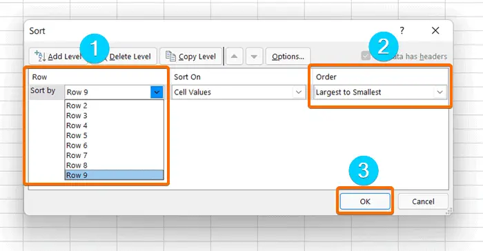
Now, select your preferred row from the Sort by drop-down.
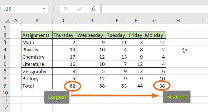
They won’t show their names, so you will need to count them. For instance, I want to sort the Total number of assignments so I picked row 9.
Then change its order from the Order drop-down. I gave it a Largest to Smallest order.

Click OK to save the changes.

And it is done! You will sort the selected rows by the desired order like in the image below, where I sorted the number of assignments of different subjects from the largest to smallest order:

Conclusion

I really hope you have a clear concept of how to sort single and multiple columns in an Excel worksheet. Following any of these techniques will help you to sort the data on your Excel sheet. But in case you have any confusion about any part of this article and face any problem sorting the columns, please feel free to mention it in the comment section.

Frequently Asked Questions

How do I bulk sort in Excel?

To bulk sort in Excel:

Click on a cell within your data range, or select the entire range you want to sort.

Press ALT + D + S sequentially to open the Sort dialog box.
In the Sort dialog box, select the column by which you want to sort under Sort by.
Optionally, add additional levels if you want to sort by multiple columns.
Choose the desired sorting order, either A to Z for ascending order or Z to A for descending order.

Check the “Preserve cell formatting” box if you want to maintain the formatting of the cells while sorting.
Once you’ve configured your sorting options, click OK to apply the sort.

This will sort the entire selected range based on the specified column(s). By following these steps, you can efficiently bulk sort data in Excel, organizing multiple rows based on your specified sorting criteria.

Can Excel filter multiple columns?

Yes, in Excel, you can use the FILTER function to filter data based on multiple columns.

Here’s an example formula: =FILTER(range, (condition1) * (condition2))

range: The range of cells you want to filter.

condition1, condition2, etc.: The conditions for each column.
Example: =FILTER(A2:C10, (B2:B10=”Category1″) * (C2:C10>50))

This formula filters the values in columns A to C based on two conditions: Column B must equal “Category1”, and Column C must have a value greater than 50. Adjust the range and conditions according to your data.

Ensure your Excel version supports the FILTER function (Excel 365, Excel 2019, Excel 2016 with updates) to use this feature.

How do you use filter formula?

To use the FILTER formula in Excel: =FILTER(range, condition)

range: The range of cells you want to filter.
condition: The condition that each cell must meet to be included in the filtered results.
Example:=FILTER(A2:A10, B2:B10=”Category1″)

This formula filters the values in cells A2 to A10 based on the condition that corresponding cells in column B are equal to “Category1”. Adjust the range and condition according to your data.

Note: The FILTER function is available in Excel 365, Excel 2019, and Excel 2016 with the latest updates. Ensure your Excel version supports this function.

Rate this post