8 VLOOKUP Limitations in Excel With Best Possible Solutions

One of the most commonly used features in Excel is the VLOOKUP function. It allows users to look up data in a table and return a corresponding value. However, while VLOOKUP is a powerful tool, it does have its limitations. In this article, I will explore the 8 limitations of VLOOKUP and offer some best possible solutions to help you overcome these limitations and make the most of your Excel spreadsheets.

1st Limitation: VLOOKUP Only Searches to the Right, Not the Left

One of the main drawbacks of the VLOOKUP function is that it only can look to the right within the table array. If the data that you want to extract is to the left of the lookup value, this function returns the #N/A error.

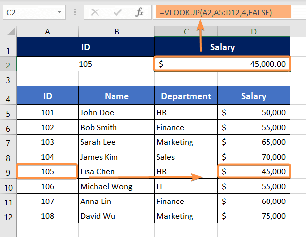
In the following scenario, I tried to look up the salary for employee id 105.

Formula

=VLOOKUP(A2,A5:D12,4,FALSE)

The VLOOKUP function just worked perfectly and returned the corresponding salary, $45,000. In this case, the data (Salary) that I wanted to extract is to the right of the lookup value (ID).

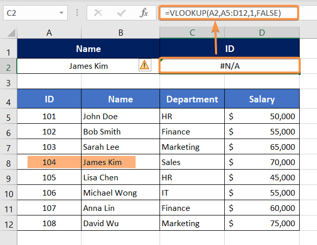
Now, let’s try the VLOOKUP function to look up the employee id corresponding to the employee name.

Formula

=VLOOKUP(A2,A5:D12,1,FALSE)

This time the VLOOKUP function fails to extract data but returns a #N/A error. In this case, the data that I wanted to look for (ID) is to the left of the lookup value (Name).

Overcoming the Limitations of VLOOKUP’s Left-to-Right Lookup

To look at both to the right and left, you can use INDEX & MATCH functions instead of the VLOOKUP function.

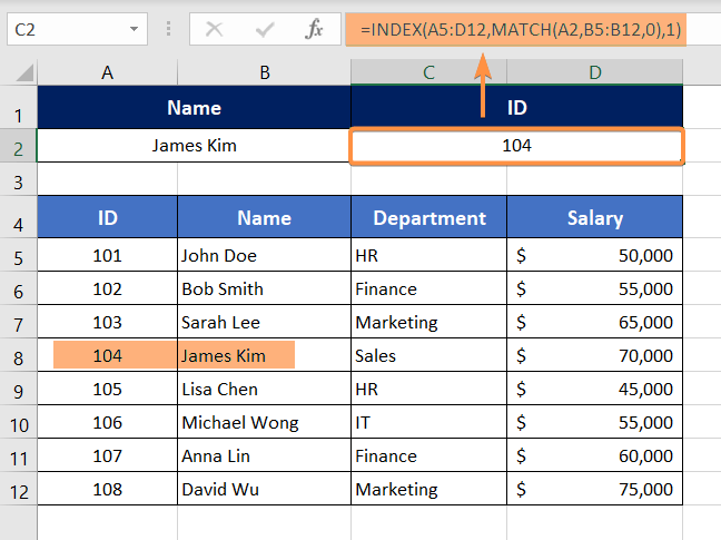
In the following scenario, I tried to extract an employee id providing an employee name as the lookup value. Here, the ID column is located to the left of the Name column.

Syntax

=INDEX(array, MATCH(lookup_value, lookup_array, [match_type]), [column_num])

Formula

=INDEX(A5:D12,MATCH(A2,B5:B12,0),1)

---

Formula Breakdown

• MATCH(A2,B5:B12,0): Here, the MATCH function looks for an exact match (referred to by 0) of James Kim (A2) within the range, B5:B12. Then, it returns the matching row number which is 4.
• So, the formula becomes INDEX(A5:D12,4,1). Now the INDEX function looks for the intersection cell of the 4th and 1st column within the table array A5:D12. The intersection cell is A8 which contains the id number, 104.
• Thus, the output of the above formula is 104.

---

2nd Limitation: VLOOKUP Can’t Lookup More Than One Column

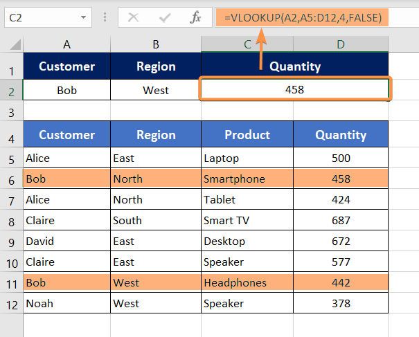
Let’s say, we want to retrieve the quantity ordered by Bob from West. Here, we have 2 customers named Bob. First Bob is from the North and second Bob is from the West.

As the VLOOKUP function can’t work based on multiple criteria, it will just retrieve data for the first lookup value (Bob from North). That’s why the output is 458.

Overcoming VLOOKUP Function’s Inability to Lookup Multiple Columns

As the VLOOKUP function cannot work with multiple criteria, we need to combine multiple columns into one column. The combined column is the helper column.

In this case, I have combined the Customer and Region columns into the Helper Column with the following formula:

Formula

=CONCAT(A5,"-",B5)

Here, I have used the CONCAT function to merge the customers’ names with their region names separated by a dash (-).

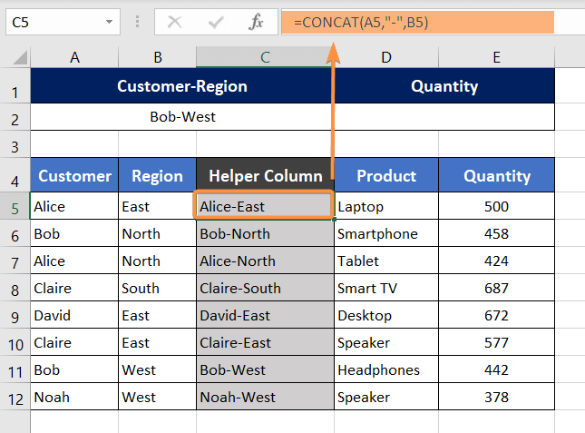
Now, I have used the Customer-Region combined data as the lookup value in the following VLOOKUP formula:

Formula

=VLOOKUP(A2,C5:E12,3,FALSE)

This time the VLOOKUP function works just fine. And it has retrieved the quantity ordered by customer Bob from West. So, the output is 442.

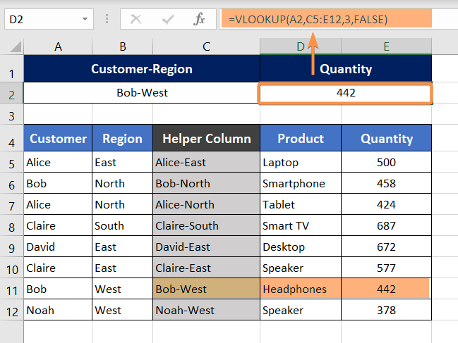
Remember, here the table array is C5:E12. So, it starts from the Helper Column. As the VLOOKUP function searches for the lookup value from the leftmost column of the table array, the range has been started from column C instead of column A.

3rd Limitation: VLOOKUP is Limited to the Left-Most Column of the Table Array

Another significant limitation of the VLOOKUP function is that it can only search for the lookup value in the leftmost column of the table array. Otherwise, it returns a #N/A error.

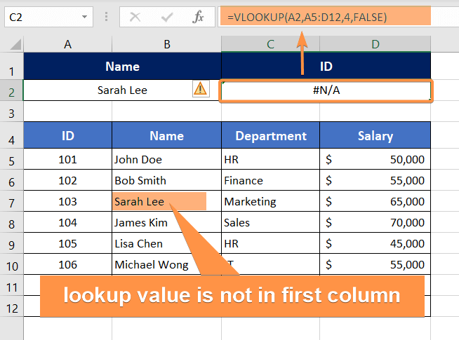
In the following dataset, the lookup value (Sarah Lee) is in the second column of the table array, A5:D12. As the lookup value is not the left-most column of the table array, it returns a #N/A error.

3 Solutions to VLOOKUP Being Restricted to the Left-Most Column of the Table Array

First Approach

If the lookup value is not in the left-most column, you need to move columns in your table to make sure that the lookup value is located in the left-most column of the table array.

Second Approach

You can change the table array in such a way that the column containing the lookup value becomes the very first column of the table array.

Third approach

Lastly, you can use the INDEX-MATCH formula to perform the search. Using this formula, you will be flexible enough with choosing the lookup value and the table array.

Formula

=INDEX(F5:I12,MATCH(F2,G5:G12,0),1)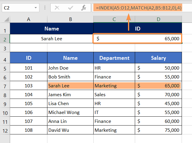

4th Limitation: VLOOKUP Isn’t Case-Sensitive

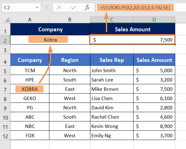
One of the primary VLOOKUP limitations is that it can’t perform a case-sensitive search. Look at the following picture, the lookup value is in the proper case (Korba). But the lookup formula returned the salary of KOBRA which is in all capitalized.

Here, Korba & KOBRA are not the same.

Overcoming the Limitation of VLOOKUP’s Case Sensitivity

To make the VLOOKUP function case-sensitive, you have to use CHOOSE & EXACT function with it.

Syntax

=VLOOKUP(TRUE, CHOOSE({1,2}, EXACT(lookup_value, lookup_array), return_array), 2, 0)

Formula

=VLOOKUP(TRUE, CHOOSE({1,2},EXACT(A2, A5:A12), D5:D12), 2, FALSE)

---

Formula Breakdown

• The first argument of the VLOOKUP function is “TRUE”, which means that the function will search for an exact match between the lookup value in A2 and the values in the first column of the table array.
• The second argument of the VLOOKUP function is a nested CHOOSE function. The CHOOSE function is used to create an array of two columns.
• =CHOOSE({1,2},EXACT(A2, A5:A12), D5:D12)
• ={FALSE,5000;FALSE,3200;FALSE,7500;FALSE,6100;FALSE,2800;FALSE,4600;FALSE,8900;FALSE,3700}
• The first column contains the results of the EXACT function, which returns TRUE if the value in A2 matches any of the values in the range A5:A12, and FALSE otherwise.
• =EXACT(A2, A5:A12)
• ={FALSE;FALSE;FALSE;FALSE;FALSE;FALSE;FALSE;FALSE}
• The second column contains the values in the range D5:D12 that correspond to each row in the first column.
• The third argument of the VLOOKUP function is “2”, which indicates that the function will return the value in the second column of the table array (i.e., column D).
• The fourth argument of the VLOOKUP function is “FALSE”, which means that the function will only return an exact match and not an approximate match.

---

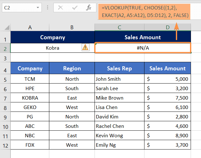
Overall, this formula is searching for an exact match between the value in cell A2 and a range of values in A5:A12 and then returns the corresponding value in column D for the row where the match is found.

5th Limitation: Slow Performance with Large Data Sets

VLOOKUP can be slow when dealing with large data sets, especially when used multiple times in the same workbook. This is because VLOOKUP has to scan through each row of the table to find the matching value, which can be time-consuming. Usually, it takes approximately 6.6 seconds to lookup through a range and 14.2 seconds for an entire column.

To improve performance, users can use alternative functions such as INDEX-MATCH or XLOOKUP that are faster and more efficient.

6th Limitation: Limited to Only One Value Per Lookup

VLOOKUP can only return one value per lookup, even if there are multiple matching values in the table. This can be a problem when dealing with duplicate values or when users want to return multiple values from the table.

Solution #1: Lookup & Return Multiple Values Using Formula

To overcome this limitation, you can use the following formula of TEXTJOIN, IF, IFERROR, MATCH, & ROW functions. This formula can return multiple values within a single cell separated by commas (,). It also automatically eliminates all duplicate values and returns the first instance of a value only.

Syntax

=TEXTJOIN(", ", TRUE, IF(IFERROR(MATCH(return_array, IF(lookup_value=lookup_array,return_array, ""), 0),"")=MATCH(ROW(return_array),ROW(return_array)),return_array, ""))

Formula

=TEXTJOIN(", ", TRUE, IF(IFERROR(MATCH(C5:C12, IF(A2=A5:A12,C5:C12, ""), 0),"")=MATCH(ROW(C5:C12),ROW(C5:C12)),C5:C12, ""))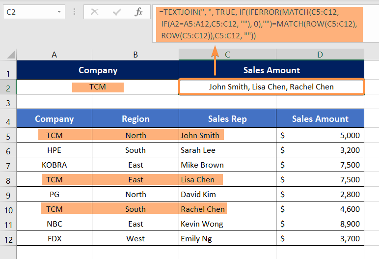

Solution #2: Lookup and Return Multiple Values Using VBA

If you don’t want to use complex formulas to return multiple values using vertical lookup, you can consider the following VBA code. This piece of code creates a user-defined function named LookupMultipleValues. This function only requires 3 arguments that are easy to use.

Function LookupMultipleValues(gTarget As String, gSearchRange As Range, gColumnNumber As Integer)

Dim g As Long
Dim k As String

For g = 1 To gSearchRange.Columns(1).Cells.Count
If gSearchRange.Cells(g, 1) = gTarget Then
For J = 1 To g - 1
If gSearchRange.Cells(J, 1) = gTarget Then
If gSearchRange.Cells(J, gColumnNumber) = gSearchRange.Cells(g, gColumnNumber) Then
GoTo Skip
End If
End If
Next J
k = k & " " & gSearchRange.Cells(g, gColumnNumber) & ","
Skip:
End If
Next g
LookupMultipleValues = Left(k, Len(k) - 1)

End Function

Usage Guide

Step_1: Press ALT + F11 to open Visual Basic Editor.

Step_2: Go to Insert > Module.

Step_3: Paste the above code.

Step_4: Return to your sheet again and use the following formula.

Syntax

=LookupMultipleValues(lookup_value,lookup_array,col_index_num)

Formula

=LookupMultipleValues(A2,A5:A12,3)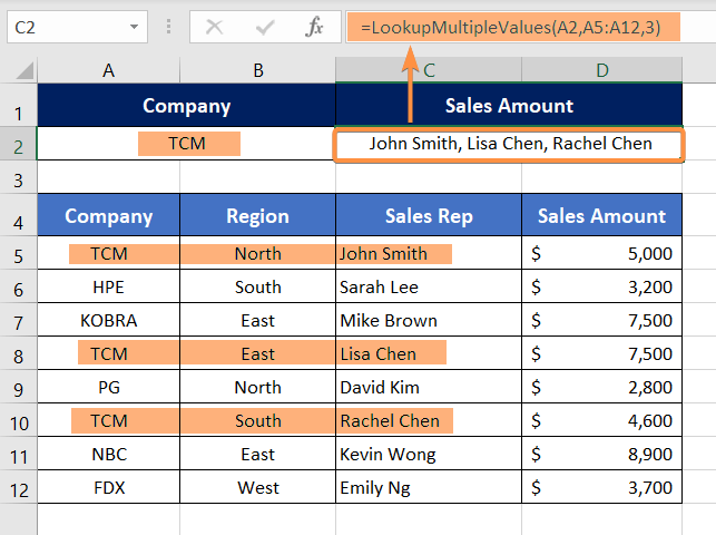

7th Limitation: VLOOKUP Function Isn’t Flexible Regarding Adding or Deleting Columns

When you insert or delete a column in the middle of your data range, it can cause issues with your VLOOKUP formula. Because the column index number that your VLOOKUP is referencing may no longer be accurate.

Usually, the 3rd argument of the VLOOKUP function i.e. column index number is hard coded. That’s why adding or removing columns within the table array may cause inaccurate results.

Resolving VLOOKUP’s Flexibility Issue Regarding Adding or Removing Columns

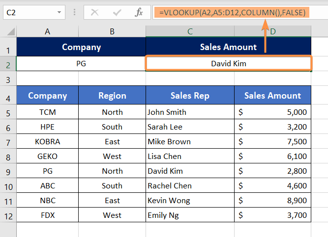
To solve this problem, you can use the COLUMN function to calculate the column index number instead of hardcoding it. For the following scenario, this is how the formula looks with and without the COLUMN function.

Static Column Index Number

=VLOOKUP(A2,A5:D12,3,FALSE)

Dynamic Column Index Number

=VLOOKUP(A2,A5:D12,COLUMN(),FALSE)

To learn more about this, you can read 2 ways to count column index number in Excel for VLOOKUP.

8th Limitation: By Default, VLOOKUP Returns Approximate Matching Results

Let’s remember the syntax of the VLOOKUP function.

Syntax

=VLOOKUP (lookup_value, table_array, col_index_num, [range_lookup])

You can see the 4th argument of the VLOOKUP function is optional. But the default setting of the range_lookup argument is TRUE – Approximate Match which is a problem. Because, if you don’t specify the range_lookup argument, it will execute an approximate match. Hence, you may not get your desired result.

If your data is not sorted, the VLOOKUP function won’t return the accurate result if the range_lookup argument is either ignored or set to TRUE- Approximate Match.

So, if you are looking for an exact match between the lookup_value and the table_array, make sure you specify the range_lookup argument as FALSE – Exact Match either by entering FALSE or 0.

Comparison Between Various Lookup Functions in Excel

Function	Advantages	Disadvantages
INDEX/MATCH	Can perform left-to-right lookups.	Longer formula syntax.
XLOOKUP	Supports approximate and exact matches.	Requires a newer version of Excel.
HLOOKUP	Can perform horizontal lookups.	Limited to only one row.
IFERROR/VLOOKUP	Can handle errors and return alternative results.	Limited to vertical lookups.
CHOOSE/MATCH	Can perform lookups based on a numeric index.	Limited to vertical lookups, less flexible than the INDEX/MATCH formula.

Conclusion

While VLOOKUP is a powerful tool for data analysis in Excel, it does have its limitations. By using the best possible solutions we’ve outlined in this article, you can overcome these limitations and take your data analysis to the next level. Whether you choose to use INDEX-MATCH, IFERROR, wildcard characters, concatenation, or helper columns, there are plenty of ways to make the most of your Excel spreadsheets and get the results you need. With a little bit of practice and experimentation, you’ll be able to master these techniques and become an Excel pro in no time.