How to Sort Horizontally in Excel [3 Methods]

To sort horizontally in Excel, follow the guide below:

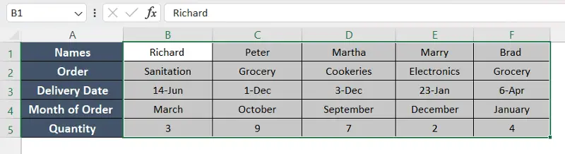
1. Select cell B7.
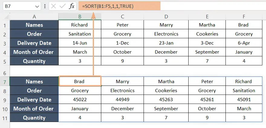
2. Write the formula: =SORT(B1:F5,1,1,TRUE)

This formula sorts a range of data B1:F5 in ascending order based on the values in the first column (column B) of the range.

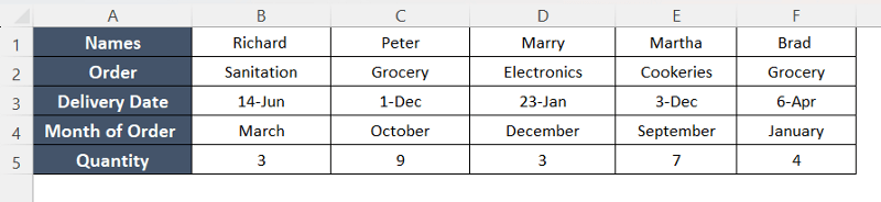
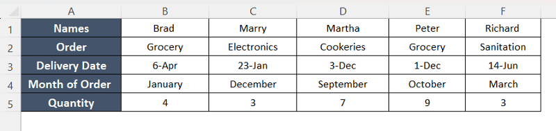
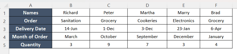
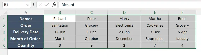
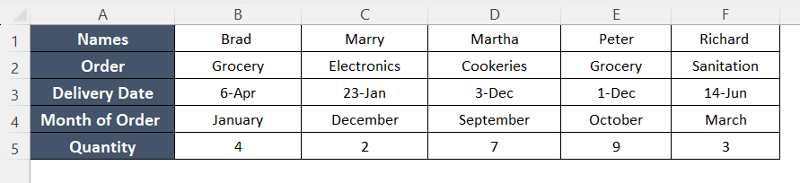
In this dataset, there are order details with the names of people who ordered, delivery date, quantity, and the months they ordered. Now we will sort the data accordingly.

Sort Horizontally by Using SORT Function in Excel

You can use the formula to sort data horizontally in Excel. Microsoft Excel in Office 365 has come up with a new dynamic function called SORT, which makes sorting in Excel much easier.

This function will let you control the range to sort, sorting order, soring index, etc. By default, it sorts data in ascending order. However, you can control it using the sort_order argument.

Syntax

=SORT(array, [sort_index], [sort_order], [by_col])

Formula

=SORT(B1:F5,1,1,TRUE)

Formula Explanation

This formula sorts the range B1:F5 based on the values in the first column (B1:B5) in ascending order, considering the first row as headers. The sorted result will be displayed in the same range.

To sort horizontally, follow the steps:

1. Copy the above formula.
2. Select cell B7 and paste it.
   
   As you can see, the “Delivery Date” is not in the date format. So you have to format the cells B9 to F9.
3. Select the cells B9:F9.
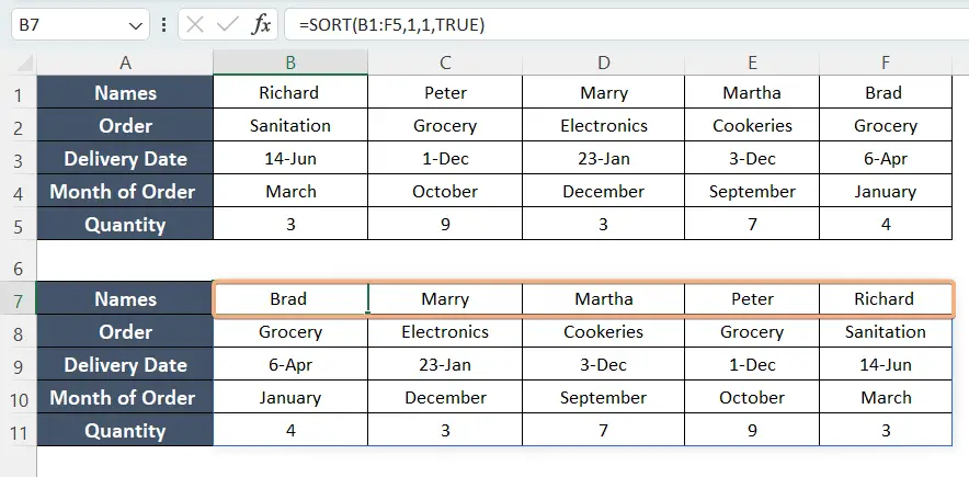
4. Press CTRL + 1 to open the Format Cells dialog box.
   
   

Here we can see the result after sorting the data horizontally.

Sort Horizontally in Excel with Custom Sort Option

To sort data horizontally, you can use the Custom Sort tool from the Editing group. Here there are some built-in features like A to Z,  Z to A, etc. However, you can customize these accordingly. If there are numbers, you can customize the data in ascending or descending order.

Sort A to Z

If you choose to sort your data by the order A to Z, you can follow the steps mentioned below.

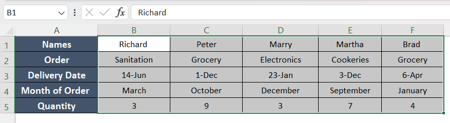
1. Select the cells that contain data for sorting.
   
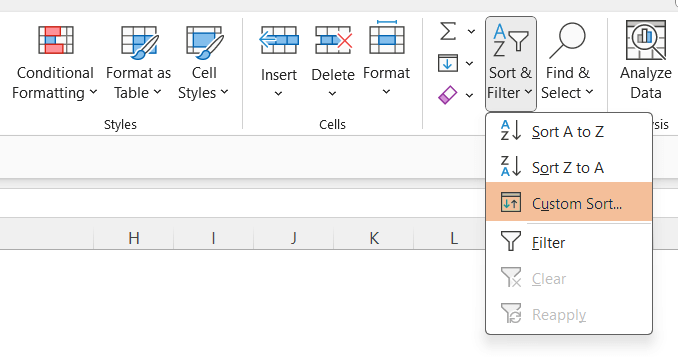
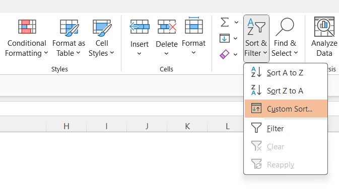
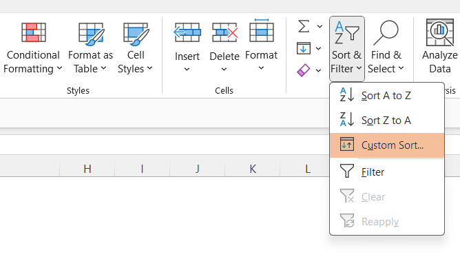
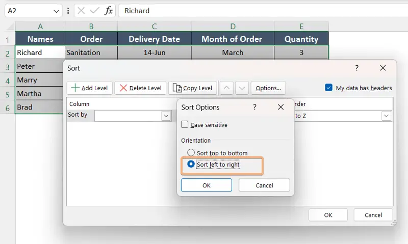
2. Go to Sort & Filter under the Editing group and select Custom Sort.
   
   
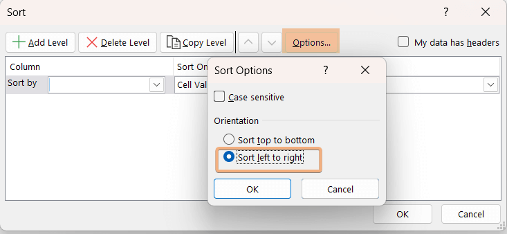
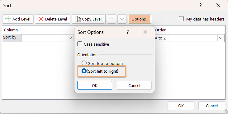
3. To sort horizontally in Excel, go to Options and then select Sort left to right.
   
   In this window, you can select the criteria for sorting.
   Here I want to sort row 1 in A to Z order.
4. Then, click OK.
   
   

Now, you can see the result. We have sorted Column A in A to Z order.

Sort Z to A

Similarly, repeat steps 1 to 3 for sorting the data in Z to A order. You just need to customize the order into Z to A instead of A to Z as the previous way.

See the change in the screenshot from the previous one. Here we sorted Column A in Z to A order.

Sort Smallest to Largest

If the cells contain numeric values, you can sort them in ascending order.
Here are the guidelines:

1. Select the cells that contain data for sorting.
   
2. Navigate to Sort & Filter under the Editing group and select Custom Sort.
   
   
3. Go to Options and then select Sort left to right to sort horizontally.
   
   
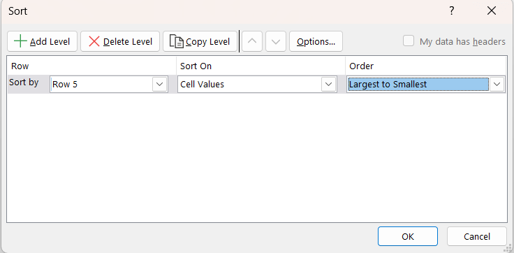
4. Row 5 contains numeric values in the dataset. Here I want to sort row 5 in the Smallest to Largest order.
5. Then click OK.
   
   

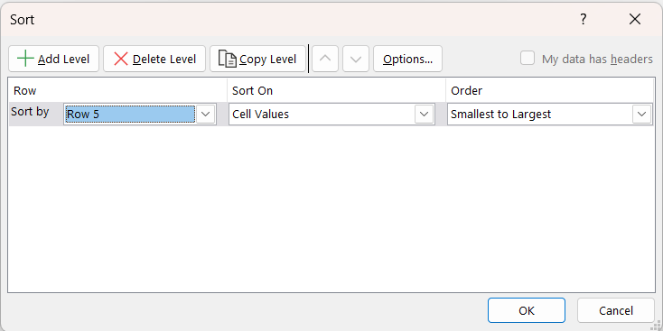
Now, you can see the sorted output in ascending order in row 5 under the header  “Quantity”.

Sort Largest to Smallest

Repeat the previous steps 1 to 3 from Sort Smallest to Largest. Now, customize the criteria for sorting. Select Largest to Smallest in the Order section. Then click OK.

Here is the result in descending order. You can notice the difference from the previous section.

Sort Multiple Rows Horizontally in Excel

To sort multiple rows horizontally, you have to follow some simple instructions.
Go through the instructions step by step:

1. To begin with, select the cells in which data are present for sorting.
   
2. Navigate to Sort & Filter in the Editing group on the Excel ribbon. Click on the Custom Sort.
   
   
3. Go to Options. As I want to sort data horizontally, I have selected Sort left to right.
   
   
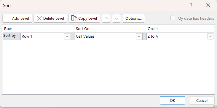
4. Now, input the criteria in each section. Here I have inputted Row 1 to sort in A to Z order. In the Sort on section, I have selected Cell Values.  To customize more rows, you can click on Add Level.
   
   Here I have added rows one by one by selecting Order with Cell Values in the Sort On section.
   

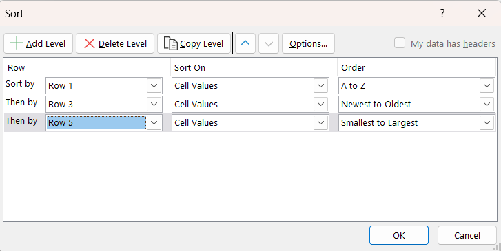
Here is the sorted result in multiple rows. We have sorted the result into row 1, row 3, and row 5.

Sort Left to Right Greyed Out in Excel

If you want to sort the cells that are part of a table, then you will see the option of Sort left to right under Custom Sort, which is greyed out.
See the image. Here is a table which I have selected to sort. I have clicked on Sort & Filter under the Editing group and selected Custom Sort.

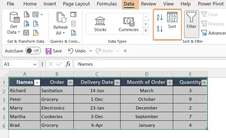
Then, to customize the Sort Options, I clicked on Options. However, it shows greyed out the option of Sort left to right.

To resolve this issue, you need to convert the table into a range. Then, go through the steps below:

1. Select the table and go to Table Design. Under the Tools group, select Convert to Range.
   
2. After that, this window will appear. Then click Yes.
   

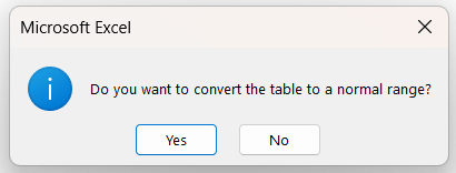
After clicking Yes, you have converted the table into the normal range. Now, go to Custom Sort and click on Options to check whether you have enabled the Sort left to right.

How to Sort Horizontally in Excel Pivot Table

A pivot table in Excel is helpful to summarize the information in a worksheet. So, it is necessary to deal with the sorting in Excel Pivot Table when working in a spreadsheet. To begin with, first, we will learn how to create a pivot table in Excel.

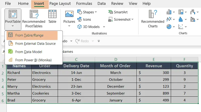
1. Select the range that contains data. Then go to the Insert tab. Now, click on the dropdown of PivotTable and select From Table/Range.
   
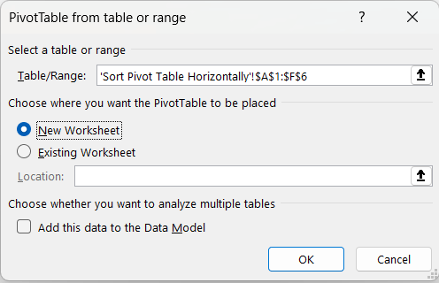
2. The previous step will lead to PivotTable from table or range. Now, choose where you want the PivotTable to be placed. Here I have selected the New Worksheet. If you want, you can choose the Existing Worksheet but in this case, you have to select range. Then, click OK.
   
   
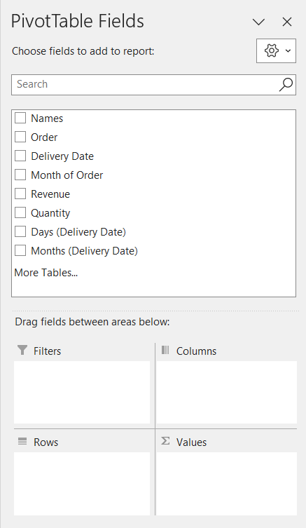
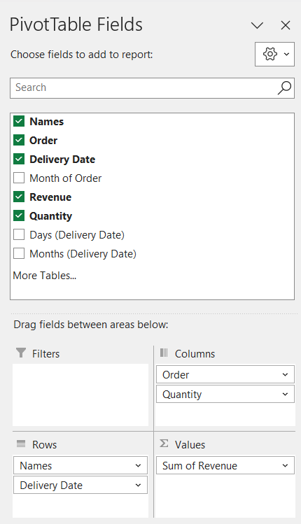
3. After clicking OK, you will see a new worksheet with PivotTable Fields on the right of the worksheet. Here you have to select the fields in four areas; Filters, Columns, Rows, and Values.
   
   Here, I have selected the “Names” and  “Delivery Date” in Rows and “Revenue” in Values, “Order” and “Quantity” in Columns.
   

Now you can see the output of sorting the column header of the pivot table horizontally. This pivot table summarizes the order and total revenue of all products with quantity. It provides a grand total of these orders as well.

Conclusion

If you are analyzing data in an Excel worksheet, you should have a strong knowledge of Excel tools. In this article, I have discussed how to sort horizontally in Excel. This tool helps you transform complex spreadsheets into more accessible and meaningful formats, enhancing your ability to analyze, report, and work with your data. If you are stuck in sorting, just go through this article and solve the issue immediately.

Frequently Asked Questions

How do you reorder rows in Excel?

To reorder rows in Excel, you can use the following steps:

1. Click on the row number on the left-hand side of the Excel sheet to select the entire row.
2. Right-click on the selected row and choose CUT from the context menu, or use the keyboard shortcut CTRL+X.
3. Click on the row number where you want to move the selected row. Ensure that the entire row is selected.
4. Right-click on the selected row and choose Insert Cut Cells from the context menu, or use the keyboard shortcut CTRL+SHIFT+“+“.

This process will cut the selected row and insert it above the row you clicked on, effectively reordering the rows.

How do I reorder columns in Excel?

To reorder columns in Excel, you can use the following steps:

1. Click on the column letter at the top of the Excel sheet to select the entire column.
2. Right-click on the selected column and choose CUT from the context menu, or use the keyboard shortcut CTRL+X.
3. Click on the column letter where you want to move the selected column. Ensure that the entire column is selected.
4. Right-click on the selected column and choose Insert Cut Cells from the context menu, or use the keyboard shortcut CTRL+SHIFT+“+“.

This process will cut the selected column and insert it to the left of the column you clicked on, effectively reordering the columns.

How do you reorder items in an Excel chart?

To reorder items in an Excel chart, follow these steps:

1. Click on the chart to select it.
2. Right-click on the chart, and choose Select Data… from the context menu.
3. In the Select Data Source dialog box, you’ll see a list of entries. To reorder them, use the up and down arrow buttons on the right side to move the selected entry.
4. Once you’ve adjusted the order, click OK to apply the changes.

This process allows you to change the order of items in the legend or the horizontal axis, affecting the visual representation of the chart.