How to Sort Data in Excel Using a Formula (7 Formulas)

Excel allows sorting your data in several ways. You can use both the Sort button as well as formulas to sort data in Excel. In this article, you will learn to sort data in Excel using a formula. Learn 7 different sorting formulas, that can help you fix any kind of sorting problem. If you are in a rush, you can check out the quick solution section to get quick help. Unfortunately, it only works in Microsoft Office 365. So without having any further discussion, let’s dive straight into them one by one.

Sort Data in Excel Using the SORT Formula

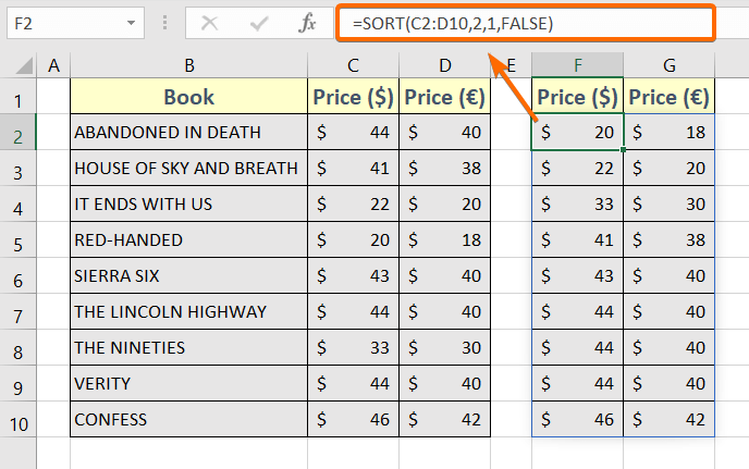
The SORT formula automates the sorting process based on specified criteria.

Formula

=SORT(C2:D10,2,1,FALSE)

Formula Explanation

• C2:D10: The range of the columns that we want to sort.
• 2: This is the sort_index.
• 1: This is responsible for sorting in ascending order. Using –1 will sort in descending order.
• FALSE: This is responsible for sorting by columns. Use TRUE to sort by rows.

To sort data in Excel using a formula, follow these steps below:

1. Select a cell to insert an array formula.
2. Use the following formula: =SORT(C2:D10,2,1,FALSE)
3. Press the ENTER button.

Attention: The SORT function is available only in Microsoft Office 365!

Sort a Single Column in Excel Having Numbers with SMALL, LARGE & ROWS Functions

Sort in Ascending Order (Sort Smallest to Largest)

Sort feature by selecting your data range and choosing the ascending order option to arrange your values from the smallest to the largest with ease.

Formula

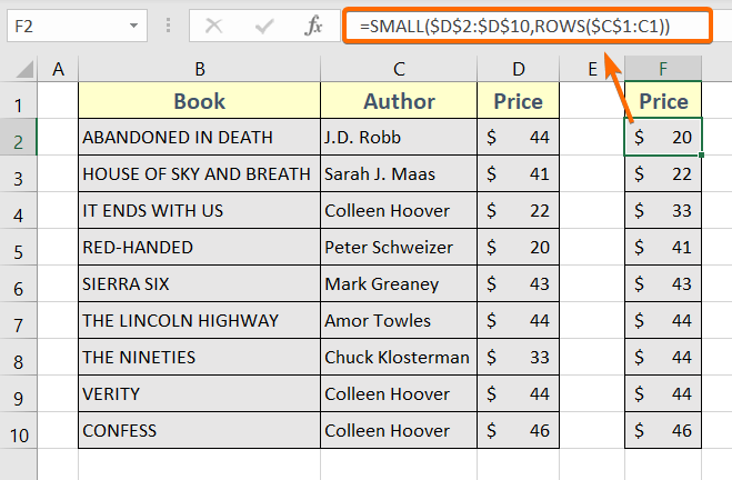
=SMALL($D$2:$D$10,ROWS($C$1:C1))

Formula Explanation

• ROWS($C$1:C1):  This returns the row count numbers such as 1,2,3, etc as you drag down the formula. Dollar signs are added to C1 to lock the cell. If you don’t lock the first cell, it will return a series of 1 only. Thus, the formula will not do its job.
• SMALL($D$2:$D$10,ROWS($C$1:C1)): This returns the first smallest number in the cell range $D$2:$D$10. As the ROWS function continues to return 2,3,4, etc respectively, then the SMALL function keeps returning the second, third, etc smallest number. Thus the numbers look sorted in ascending order.

To sort a single column with the SMALL function, follow these steps below:

1. Create a separate column where you want to get your numbers sorted.
   I made a separate column called Price in column F.
2. Now, insert the following formula in the first cell (Cell F2) of the new column: =SMALL($D$2:$D$10,ROWS($C$1:C1))
3. After that, hit the ENTER button to execute the formula.
4. Now, place your mouse curse in the right bottom corner of cell F2. The Fill Handle icon will appear.
5. Drag the Fill Handle icon from cell F2 to F10.
   This will apply the above formula from cell F2 to F10.

Sort in Descending Order ( Sort Largest to Smallest)

Access the Sort feature, and choose the descending order option to quickly organize your values from the largest to the smallest.

Formula

=LARGE($D$2:$D$10,ROWS($C$1:C1))

Formula Explanation

• $D$2:$D$10: This is the range of the cells where the numbers are located. You need to update this as per your datasheet.
• $C$1:C1: This is the row counter. You can keep this intact in your formula. Or, you can modify this but always use the same cell address here with the first part of it locked.

Use the LARGE function to sort in descending order. To do that, follow the steps below:

1. Create a separate column to store the formula result.
   I made another column named Price in column F.
2. Insert the following formula in the first cell of the new Price column.
3. Hit ENTER to execute the formula.
4. Drag the Fill Handle icon from cell F2 to F10 to apply the same formula all around this cell range.

• How to Sort Multiple Columns in Excel (4 Techniques)

Sort a Single Column in Excel Having Numerical Values with SMALL, LARGE, and ROW Functions

Sort in Ascending Order Using the Array Formula (Sort Smallest to Largest)

Sort your data in ascending order using an array formula to arrange values from the smallest to the largest in Excel.

Formula

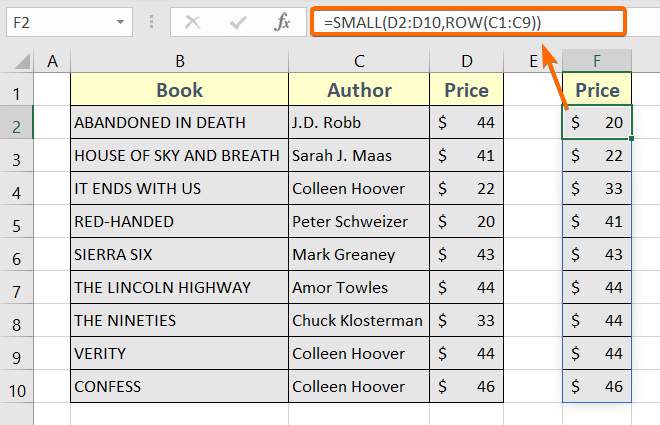
=SMALL(D2:D10,ROW(C1:C9))

Formula Explanation

• D2:D10 is the cell range where the numbers are stored.
• C1:C9 is used to return a row count number. You should always make the count equal to the number of rows in your data table. For example, if you have 50 rows in your data table, it will be C1:C49. You can other cell addresses here such as A1:A9, B1:B9, C1:C9, etc.

To sort data in ascending order with an array formula, here are the steps:

1. Create a new column to store the formula result.
2. Enter the following array formula in the first cell of the newly created column: =SMALL(D2:D10, ROW(C1:C9))
3. If you are using Microsoft Office 365, just press the ENTER button to execute.
   For the other versions of MS Excel, select the whole new column > insert the above formula in the first cell of the selected cells > press CTRL + SHIFT + ENTER to insert the array formula.

Sort in Descending Order Using Array Formula ( Sort Largest to Smallest)

Sort your data in descending order, arranging values from the largest to the smallest, in Excel by leveraging array formulas.

Formula

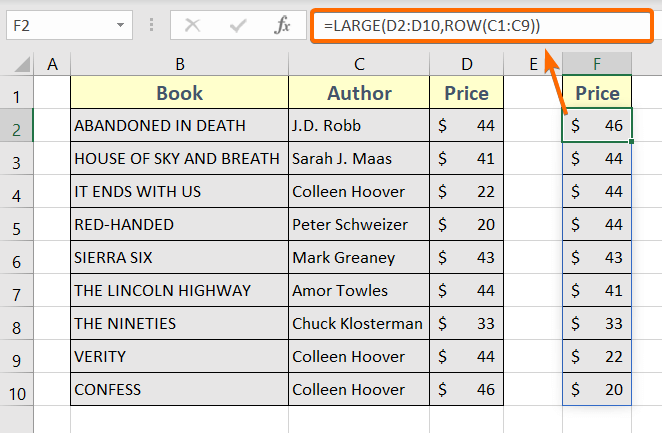
=LARGE(D2:D10,ROW(C1:C9))

Formula Explanation

• D2:D10 is the cell range where the numbers are stored.
• C1:C9 is used to return a serial number equal to the total row numbers in the data table starting from 1.

Steps to sort data in descending order with an array formula:

1. Create a new column to store the sorted numbers.
2. Insert the following formula in the very first cell of the new column: =LARGE(D2:D10,ROW(C1:C9))
3. If you are using Microsoft Office 365, just press the ENTER button to execute.
   For the other versions of MS Excel, select the whole new column > insert the above formula in the first cell of the selected cells > press CTRL+SHIFT+ENTER to insert the array formula.

• How to Sort in Excel by Name (3 Techniques)

Sort a Single Column in Excel with Text Using INDEX, MATCH, ROWS, and COUNTIF Functions

Sort in Ascending Order (Sort A to Z)

You can combine INDEX, MATCH, ROWS, and COUNTIF functions in ascending order to sort a single column in Excel having text.

Formula

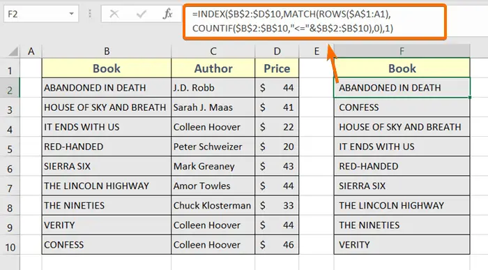
=INDEX($B$2:$D$10,MATCH(ROWS($A$1:A1),COUNTIF($B$2:$B$10,"<="&$B$2:$B$10),0),1)

Formula Explanation

• $B$2:$D$10 is the table range. You need to update this range according to your data table.
• $A$1:A1 is used to return the row number counts such as 1, 2, 3, etc. You can use anything like $B$1:B1, $C$1:C1, $D$1:D1, etc here.
• $B$2:$B$10 is the range of the cells where the text data are stored. You need to update this range as per your data table.
• <= is responsible for sorting data from A to Z. If you change this operator to >=, it will sort data from Z to A.
• 0 is used to define an Exact Match. You can leave this option as it is.
• 1 is the column index number. This means the range $B$2:$B$10 is the first column of the table range $B$2:$D$10. You must update this according to your data table. You can use 2 to indicate the second column, 3 for the third column, etc.

Steps to sort a single column in Excel having text in ascending order:

1. Create a new column to store the sorted texts.
2. Insert the following formula in the first cell of the new column: =INDEX($B$2:$D$10,MATCH(ROWS($A$1:A1),COUNTIF($B$2:$B$10,”<=”&$B$2:$B$10),0),1)
3. Now, press the ENTER button to finish inserting it.
4. Drag the Fill Handle icon from cell F2 to F10.

Sort in Descending Order ( Sort Z to A)

Steps to sort a single column in Excel having text in descending order combining INDEX, MATCH, ROWS, and COUNTIF functions:

1. Create a new column to store the sorted data.
2. Insert the following formula in the very first cell of the newly created column: =INDEX($B$2:$D$10,MATCH(ROWS($A$1:A1),COUNTIF($B$2:$B$10,”>=”&$B$2:$B$10),0),1)
3. Hit ENTER.
4. Drag the Fill Handle icon to the end of the new column.

• How to Sort by Number in Excel (4 Techniques)

Sort a Single Column in Excel Having Texts Using the INDEX, MATCH, ROW, and COUNTIF Functions

Sort in Ascending Order (Sort A to Z)

Apply a formula utilizing the INDEX, MATCH, ROW, and COUNTIF functions to create a sorted array in ascending order.

Formula

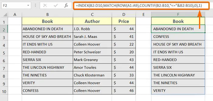
=INDEX(B2:D10,MATCH(ROW(A1:A9),COUNTIF(B2:B10,"<="&B2:B10),0),1)

Formula Explanation

• B2:D10 is the data table range. You will update this range.
• A1:A9 is used to return 1, 2, 3…10, as there is a total of 10 rows in the data table. Here, you can use anything like B1:B9, C1:C9, D1:D9, etc.
• B2:B10 is the cell range of the column where the text data are stored. You need to update this range.
• <= is responsible for sorting data in ascending order. You can use >= to sort in descending order.
• 0 is used to define an Exact Match. In general, you need not update this.
• 1 is a column index number. This means range B2:B10 is the 1st column of the table range B2:D10. You can use 2,3,4, etc to refer 2nd, 3rd, and 4th columns respectively.

Apply a formula with multiple functions to sort in ascending order. Here’s how:

1. First of all, create a new column to store the sorted data.
2. Enter the following array formula in the first cell of the new column:=INDEX(B2:D10,MATCH(ROW(A1:A9),COUNTIF(B2:B10,”<=”&B2:B10),0),1)
3. For Microsoft Office 365, just hit the ENTER button to insert the formula.
   For the Other versions of Excel users, Select an equal number of cells as the source column > in the first cell of the selection range, insert the above formula > press CTRL+SHIFT+ENTER to insert the above array formula.

Sort in Descending Order ( Sort Z to A)

Create a formula with INDEX, MATCH, ROW, and COUNTIF functions in descending order.

Formula

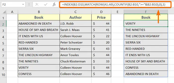
=INDEX(B2:D10,MATCH(ROW(A1:A9),COUNTIF(B2:B10,">="&B2:B10),0),1)

To sort data in descending order (Z to A) using INDEX, MATCH, ROW, and COUNTIF in Excel, you can create a formula. So, follow these steps below:

1. Create a new column to store the sorted text data.
2. Use the following array formula in cell F2, which is the first cell of the new column.
3. For Microsoft Office 365, just hit the ENTER button to insert the formula: =INDEX(B2:D10,MATCH(ROW(A1:A9),COUNTIF(B2:B10,”>=”&B2:B10),0),1)
   For the Other versions of Excel users, Select an equal number of cells as the source column > in the first cell of the selection range, insert the above formula > press CTRL+SHIFT+ENTER to insert the above array formula.

• How to Sort in Excel by Date (3 Ways)

Sort Data in Excel Using the SORT Function (Single & Multiple Columns)

The SORT function is available only in Microsoft Office 365.

//If you are using an older version of Excel, you can’t use this formula.

SORT Function Syntax

=SORT (table_array, [sort_index], [sort_order], [by_col])

Function Arguments

• table_array:This field is mandatory. Here, you will insert the cell range of a single column or multiple columns to sort their contents.
• sort_index : This is optional to insert. By default, the value is set to 1. Here, you will insert the column number of the table array based on which the data will be sorted.
• sort_order: This is also an optional field. It has two values.  Value 1 is for sorting in an ascending and -1 is for sorting in descending order. The default value is 1.
• by_col: This is also optional. Its value can be either TRUE or FALSE. If you want to sort by the column you will insert TRUE. To sort by row you will insert FALSE. But by default, its value is set to FALSE.

Sort in Ascending Order (Sort Smallest to Largest)

To sort data in ascending order (smallest to largest) in Excel, you can use the SORT function.

Formula

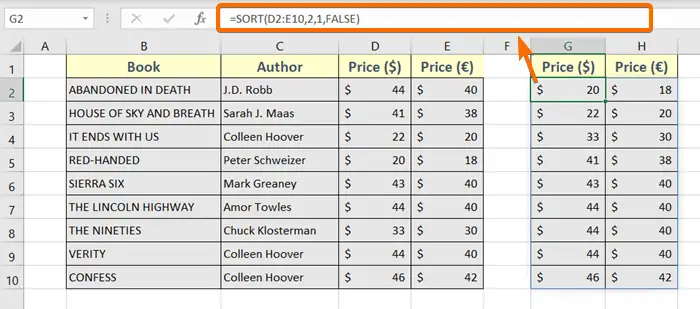
=SORT(D2:E10,2,1,FALSE)

Formula Explanation

• D2:E10 is the range of the columns that we want to sort.
• 2 is the sort_index.
• 1 is responsible for sorting in ascending order.
• FALSE is responsible for sorting by columns.

Now, follow these steps to apply the SORT function to sort in ascending order:

1. Allocate cells where you want to keep the sorted data.
2. Insert the following formula in the first cell of the selected space: =SORT(D2:E10,2,1,FALSE)
   In this case, it’s cell G2.
3. Just hit the ENTER button to insert the formula.

Sort in Descending Order ( Sort Largest to Smallest)

To sort data in descending order (largest to smallest) in Excel, you can use the SORT function.

Formula

=SORT(D2:E10,2,-1,FALSE)

Formula Explanation

• D2:E10 is the range of the columns that we want to sort.
• 2 is the sort_index.
• -1 is responsible for sorting in descending order.
• FALSE is responsible for sorting by columns.

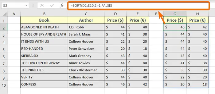
Here are the steps to sort data in descending order with the SORT function:

1. Create separate columns as per the requirement to store the sorted data.
2. Insert the following formula in the very first cell of the newly created columns, cell G2: =SORT(D2:E10,2,-1,FALSE)
3. Now, hit the ENTER button to execute the above formula.

• How to Sort in Excel by Color (3 Techniques)

Sort Multiple Columns in Excel Having Numbers Using the INDEX, MATCH, ROW, LARGE, and SMALL Functions

Sort in Ascending Order (Sort A to Z)

Combine INDEX, MATCH, ROW, LARGE, and SMALL functions to sort multiple columns with numbers in Excel.

Formula

=INDEX(D2:E10,MATCH(SMALL(D2:D10,ROW(A1:A9)),D2:D10,0),MATCH(G1:H1,G1:H1,0))

Formula Explanation

• D2:E10 is the range of the cells, whose contents you want to sort.
• D2:D10 is the cell range of the first column of the considered table array, D2:E10.
• A1:A9 returns the row count value. It returns serial numbers from 1 to 9. This series of numbers should be equal to the number total number of rows in the data table. In this case, the total number of rows in the range D2:E10 is 10. That’s why A1:A9 was taken. This should always start from cell 1 such as A1, B1, C1, etc.
• 0 defines the Exact Match type.
• G1:H1 is the very first-row range of the newly created table to store the sorted data.

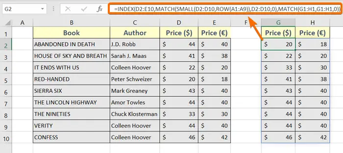
To sort multiple columns having numbers in ascending order, go through these steps below:

1. Allocate space to store the sorted numbers.
2. Insert the following formula in the first cell of the newly allocated space, cell G2: =INDEX(D2:E10,MATCH(SMALL(D2:D10,ROW(A1:A9)),D2:D10,0),MATCH(G1:H1,G1:H1,0))
3. Now, if you are using Microsoft Office 365, just press the ENTER button to execute.
   For the other versions of MS Excel, select the range G2:H10 > insert the above formula in the first cell of the selected cells > press CTRL+SHIFT+ENTER to insert the array formula.

Sort in Descending Order ( Sort Z to A)

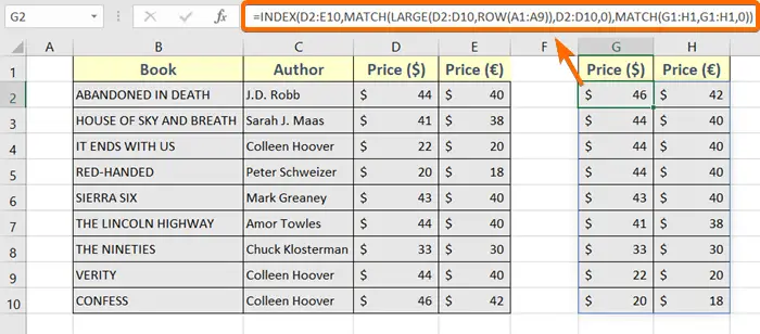
If you replace the SMALL function in the formula of the previous method, it will sort numbers in descending order. Anyway, here is the full process for you:

1. First, create a blank table with headers like columns D & E in columns G & H.
2. Then, insert the following formula in cell G2: =INDEX(D2:E10,MATCH(LARGE(D2:D10,ROW(A1:A9)),D2:D10,0),MATCH(G1:H1,G1:H1,0))
3. Now, if you are using Microsoft Office 365, just press the ENTER button to execute.
   For the other versions of MS Excel, select the range G2:H10 > insert the above formula in the first cell of the selected cells > press CTRL+SHIFT+ENTER to insert the array formula.

Sort Multiple Columns in Excel Having Texts Using the INDEX, MATCH, ROW, and COUNTIF Functions

Sort in Ascending Order (Sort Smallest to Largest)

Use INDEX, MATCH, ROW, and COUNTIF functions to sort multiple columns having texts in Excel.

Formula

=INDEX(B2:C10,MATCH(ROW(A1:A9),COUNTIF(B2:B10,"<="&B2:B10),0),MATCH(F1:G1,F1:G1,0))

Formula Explanation

• B2:C10 is the range of the source data table.
• A1:A9 is the row number counter.
• B2:B10 is the first column of the source data table.
• <= is responsible for sorting in ascending order.
• 0 defines an Exact Match.
• F1:G1 is the first row of the newly created blank table.

Steps to sort multiple columns having texts in Excel:

1. Create a blank table just like the one whose contents you want to get sorted.
2. Insert the following formula in the first cell of the blank table. Cell G2 for this case.
3. Now, if you are using Microsoft Office 365, just press the ENTER button to execute.
   For the other versions of MS Excel, select the range F2:G10 > insert the above formula in the first cell of the selected cells >press CTRL+SHIFT+ENTER to insert the array formula.

Sort in Descending Order ( Sort Largest to Smallest)

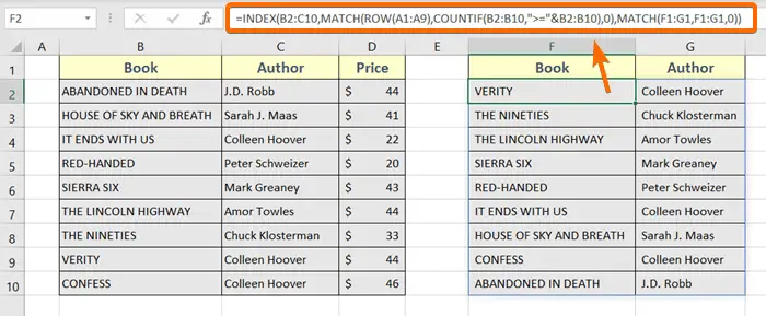
This is the same formula as the formula used in the previous method. Just the “<=” is replaced by “>=”. To use the formula, follow these steps below:

1. First of all, allocate a cell range to store the formula result.
2. Insert the following formula in the very first cell of the allocated cell range, cell F2: =INDEX(B2:C10,MATCH(ROW(A1:A9),COUNTIF(B2:B10,”>=”&B2:B10),0),MATCH(F1:G1,F1:G1,0))
3. Now, if you are using Microsoft Office 365, just press the ENTER button to execute.
   For the other versions of MS Excel, select the range F2:G10 > insert the above formula in the first cell of the selected cells > press CTRL+SHIFT+ENTER to insert the array formula.

Conclusion

So, we have discussed 7 different formulas to sort data in Excel. Each of the formulas has its purpose while sorting data in Excel. If you face any problems using any of the formulas, let us know in the comment section. We will try to help you ASAP.

Frequently Asked Questions

How do I automatically sort data in Excel?

To automatically sort data in Excel:

1. Highlight the column or range of data you want to sort.
2. Navigate to the Data tab in the Excel ribbon.
3. Find and click on the Sort button.
4. In the Sort dialog box, select the column by which you want to sort and specify the sorting order.
5. Once you’ve configured your sorting options, click OK to apply the sort.

For automatic sorting upon changes or additions, consider using Excel Tables (Insert > Table) and enabling the Sort and Filter options. This ensures that new data is automatically included in the sorting process.

How do you categorize data in Excel using the IF formula?

To categorize data in Excel using the IF formula, follow these steps:

1. Choose a cell where you want the categorized result to appear.
2. Enter a formula like: =IF(logical_test, “Category1”, “Category2”)
   Replace “logical_test” with the condition you want to evaluate.
3. Hit ENTER to see the category based on the logical test. Example: =IF(A2>10, “High”, “Low”)
   This formula categorizes the value in cell A2 as “High” if it’s greater than 10; otherwise, it’s categorized as “Low”.

Use the IF formula to dynamically categorize data based on specified conditions in Excel. Adjust the conditions and categories to suit your specific dataset and criteria.