How to Use TYPE Function in Excel [3 Examples]
What Does the Excel TYPE Function Do?
The TYPE function serves a fundamental purpose: it enables users to determine the data type of a specified value in Excel. Whether you’re working with numbers, text, logical values, or error values, this function helps identify the underlying data type, aiding in data analysis and manipulation tasks.
What is the Syntax of the TYPE Function?
The syntax of the TYPE function is straightforward, comprising a single argument in Excel:
=TYPE(value)Here, “value” represents the data point for which you want to ascertain the data type.
What Are the Arguments of the Excel TYPE Function?
The TYPE function accepts one argument:
- value: This mandatory argument denotes the value or reference whose data type you wish to identify. It can be a cell reference, a numerical value, a text string, or any other valid Excel value.
What is the Output of the TYPE Function?
The output of the TYPE function is a numeric code corresponding to the data type of the specified value in Excel. These codes range from 1 to 16, each representing a different data type. Understanding these codes is crucial for interpreting the results accurately.
3 Examples of Using the TYPE Function in Excel
Example 1: Determining the Data Type of a Numeric Value
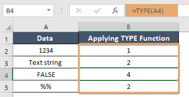
Suppose cell A2 contains the value 1234. To ascertain its data type, you can use the following formula:
=TYPE(A2)The result will be 1, indicating that the value in cell A2 is numeric.
Example 2: Identifying the Data Type of a Text String
If cell A3 contains the text “Text String”, you can determine its data type with the following formula:
=TYPE(A3)The output will be 2, signifying that the value in cell A3 is a text string.
Example 3: Analyzing Logical Values
For a logical value such as TRUE or FALSE in cell A4, the TYPE function yields:
=TYPE(A4)The returned value will be 4, indicating a logical value.

Things to Remember
- The TYPE function is case-insensitive.
- Error-values such as #N/A or #DIV/0! have specific numeric codes.
- The function returns an error if the input value is an array.
Conclusion
Mastering the TYPE function empowers users to efficiently analyze and manipulate data by accurately identifying the data types of various values within a spreadsheet. By understanding its syntax, arguments, and output, you can leverage this function to streamline your data management processes and enhance your productivity in Excel.
Frequently Asked Questions
Can the TYPE function handle arrays?
No, the TYPE function cannot process arrays as input. It only accepts single values or cell references in Excel.
What does a return value of 16 signify?
A return value of 16 indicates an error value, such as #N/A or #DIV/0!.
Is the TYPE function case-sensitive?
No, the TYPE function is case-insensitive, which treats uppercase and lowercase characters as identical when identifying text strings in Excel.
Can I use the TYPE function in combination with other functions in Excel?
Yes, you can combine the TYPE function with other functions to perform more complex data analysis tasks in Excel. For instance, you can use it within logical functions like IF to conditionally process data based on its type.