How to Return Array Using XLOOKUP in Excel[4 Methods]

To return the array using the XLOOKUP function, follow the steps below:

1. Select cell B11.
2. Write down this formula:=XLOOKUP(A11,A2:A8,B2:D8,””)
3. Click the ENTER key.

It can be especially useful when you need to search for specific values in a table and extract related information, such as looking up a product name and returning its associated price and company name.

Example 1: Using XLOOKUP Function to Return Array

XLOOKUP is a powerful and versatile lookup function introduced in Microsoft Excel, primarily designed for data retrieval and lookup tasks. It can perform both vertical and horizontal lookups.This function is particularly useful for performing exact or approximate matches and allows for a more versatile data retrieval process compared to traditional lookup functions, such as VLOOKUP.

Syntax

=XLOOKUP(lookup_value,lookup_array,return_array,[if_found_matches])

Formula

=XLOOKUP(A11,A2:A8,B2:D8,"")

Formula Breakdown

This formula in Excel searches for the value in cell A11 within the range A2:A8, and when it finds a match, it returns the corresponding value from the range B2:D8. If no match is found, it returns an empty cell (“”).

Follow these steps to return array, by using XLOOKUP function:

1. Select cell B11.
2. Write down this formula:=XLOOKUP(A11,A2:A8,B2:D8,””)
3. Click the ENTER key.

Final Result

After searching for the product name ‘S 23 Ultra,’ it returned an array of associated values, including ‘Company Name,’ ‘Operating System,’ and ‘Price’.

Example 2: Using the Combination of CHOOSECOLS and XLOOKUP Function to Return Selected Columns

You can combine the CHOOSECOLS and XLOOKUP functions to retrieve particular columns as an array. The CHOOSECOLS function serves the purpose of selecting and returning specific columns within an Excel sheet.

Syntax

=CHOOSECOLS(XLOOKUP(lookup_value,lookup_array,return_array,[if_found_matches]),col_num_1,[col_num_2])

Formula

=CHOOSECOLS(XLOOKUP(A11,A2:A8,B2:D8,""),1,3)

Formula Breakdown

This formula first uses the XLOOKUP function to search for the value in cell A11 within the range A2:A8.

• When it finds a match, it returns the corresponding row as an array from the range B2:D8, or an empty cell if no match is found.
• Then, it utilizes the CHOOSECOLS function, which selects specific columns from the resulting array. In this case, it chooses columns 1 and 3, meaning it returns the values from the first and third columns of the matched row.

Use the combination of CHOOSECOLS and XLOOKUP functions to return selected columns, Here how it’s work:

1. Choose cell B11.
2. Write this formula: =CHOOSECOLS(XLOOKUP(A11,A2:A8,B2:D8,””),1,3)
3. Hit ENTER to see the result.

Final Result

This formula is useful for selectively extracting data from a table based on the lookup value and the desired columns.

Example 3: Using the Combination of XLOOKUP and FILTER Functions to Return Array for Multiple Match

You can achieve this by using a combination of the XLOOKUP and FILTER functions to not only return arrays but also retrieve data when multiple matches are found.

Syntax

=FILTER(array, XLOOKUP(lookup_value,lookup_array,return_array,[if_found_matches]))

Formula

=FILTER(B2:D8, XLOOKUP("*" & A11 & "*",A2:A8,A2:A8,"",1)=A2:A8)

Formula Breakdown

This formula in Excel filters a range of data (B2:D8) based on a two-step lookup process.

• First, it uses XLOOKUP to search for the value in cell A11, with wildcards added to perform partial matching, within the range A2:A8, and returns an array of results.
• Then, it checks whether each corresponding value from the XLOOKUP result matches the values in the range A2:A8.
• If there’s a match, the entire row from the original data range B2:D8 is included in the filtered result.

This formula is especially helpful for extracting data where the name in A11 partially matches the names in the data, and it returns rows that meet the specified criteria.

After following the steps below, you can easily return multiple matches by using the combination of XLOOKUP and FILTER functions:

1. Select cell B11.
2. Type this formula:=XLOOKUP(A11,A2:A8,B2:D8,””)
3. Press ENTER to see the result.

Final Result

When searching for ‘Android’ in the ‘Operating System’ column, it returns an array of all Android devices.

Example 4: Using the Combination of CHOOSE, XLOOKUP, and FILTER Functions to Return Selected Columns for Multiple Match

You can achieve this by using a combination of the CHOOSE, XLOOKUP, and FILTER functions to return specific columns when multiple matches are found.

Syntax

=CHOOSE({1,2}, FILTER(B2:B8, XLOOKUP(lookup_value,lookup_array,return_array,[if_found_matches])), FILTER(D2:D8, XLOOKUP(lookup_value,lookup_array,return_array,[if_found_matches])))

Formula

=CHOOSE({index_num}, FILTER(array, XLOOKUP("*" & A11 & "*", A2:A8, A2:A8, "", 1) = A2:A8), FILTER(array, XLOOKUP("*" & A11 & "*", A2:A8, A2:A8, "", 1) = A2:A8))

Formula Breakdown

It is used to perform a complex data retrieval operation.

• It begins with XLOOKUP, which searches for the value in cell A11 with wildcard characters for partial matching within the range A2:A8. This results in an array of TRUE/FALSE values based on the match condition.
• FILTER is then used twice to filter two separate columns: one for “Product Names” (B2:B8) and another for “Company Names” (D2:D8). The TRUE/FALSE array from the XLOOKUP determines which rows are included in the filtered results.
• Finally, CHOOSE is employed to select and return two separate arrays of “Product Names” and “Company Names” based on the condition.

This complex formula effectively retrieves product and company names where the name in A11 partially matches the names in column A2:A8.

You may quickly return multiple matches by using the CHOOSE, XLOOKUP, and FILTER functions as shown in the steps below:

1. Choose cell B11.
2. Type this formula:=XLOOKUP(A11,A2:A8,B2:D8,””)
3. Press the ENTER button.

Final Result

Using this formula, you can efficiently retrieve multiple matches and return them as an array.

Alternative Way to Return Array Without Using the XLOOKUP Function

You can also use the FILTER function to return an array without using the XLOOKUP function.

Syntax

=FILTER(array,include,[if_empty])

Formula

=FILTER(B2:C8,D2:D8=A11," ")

Formula Breakdown

This formula in Excel is used for filtering data in a table.

• It checks the values in the range D2:D8 to see if they are equal to the value in cell A11. This creates a TRUE/FALSE array where TRUE represents rows in which the values in D2:D8 match the value in A11.
• The FILTER function then selects and returns the corresponding rows from the range B2:C8 where the condition is met, effectively displaying the data from columns B and C for the rows that satisfy the condition.
• The empty string (” “) is used as a placeholder value and does not impact the filtering process; it can be replaced with specific criteria or left empty based on the desired filtering condition.

To return array without using the XLOOKUP function, follow these steps below:

1. Choose cell B11.
2. Type this formula:=FILTER(B2:C8,D2:D8=A11,” “)
3. Press the ENTER button.

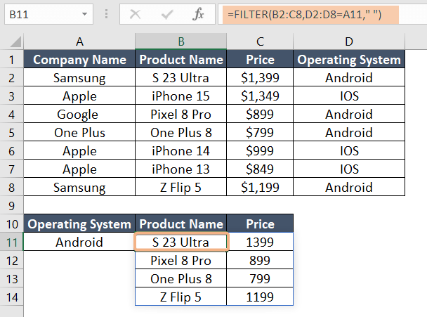
Final Result

Conclusion

XLOOKUP is a versatile Excel function for searching and retrieving data. It simplifies complex lookup operations and offers more flexibility compared to older functions. By following these four examples, you’ll learn how to use XLOOKUP to retrieve arrays of data, including situations with multiple matches.

Frequently Asked Questions

What is the return array in Xlookup?

In the XLOOKUP function in Excel, the return array is the range of data where Excel looks for the answer. When you search for something, XLOOKUP checks a specific place, like a book index, to find where your answer is.

Once it finds the answer, it returns the information from that same place in the return array. It’s like finding a word in a dictionary and then reading the definition on the same page. The return array is where Excel gets the answer to give back to you.

Is Xlookup better than VLOOKUP?

Yes, XLOOKUP is generally better than VLOOKUP in Excel. XLOOKUP is more flexible and can search in both vertical and horizontal directions, while VLOOKUP only searches vertically.

XLOOKUP simplifies the syntax, making it easier to use, and provides improved error-handling options. It can return multiple values as an array, which is often more practical, and it’s considered the preferred choice for modern Excel users due to its versatility and user-friendliness.

What does the Xlookup function return?

The XLOOKUP function in Excel is used for searching a range or array, and it returns the corresponding value of the first match it finds. The function is versatile and includes additional features compared to its predecessors, such as VLOOKUP and HLOOKUP. The XLOOKUP function can return a specific value, an array of values, or even perform approximate matches.

Here is a basic syntax for the XLOOKUP function:

XLOOKUP(lookup_value, lookup_array, return_array, [if_not_found], [match_mode], [search_mode])

Can VLOOKUP return an array?

The VLOOKUP function in Excel is designed to return a single value based on a lookup. By default, it returns the value in a specific column of the table array where it finds the first match for the lookup value.

However, if you want to retrieve multiple values based on a single lookup value, you can use an array formula with VLOOKUP combined with functions like IF, INDEX, and MATCH. This technique is commonly referred to as an “array formula.”

Can Hlookup return an array?

Similar to VLOOKUP, the HLOOKUP function in Excel is designed to look up a value in the first row of a table and return a corresponding value from a specified row. By default, it returns a single value based on the lookup.

However, if you want to retrieve multiple values based on a single lookup value, you can use an array formula with HLOOKUP combined with functions like IF, INDEX, and MATCH.