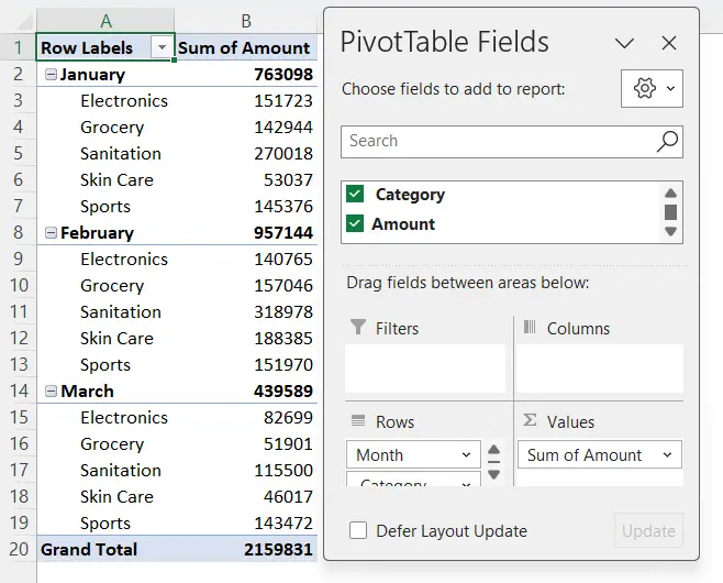
3 Ways to Create Pivot Table from Multiple Sheets in Excel

There are some cases where you have distributed data in multiple sheets. You will need to create a pivot table from multiple sheets in Excel. For example, you have 3 months of sales reports in three different sheets. However, you want to append them together to work on the sales, such as best-selling, employee performance, etc. In this scenario, you will have to create multiple sheets in Excel. In this article, I have discussed 3 methods to create a pivot table in Excel. So, let’s start.

Table of Contents

Create Pivot Table from Multiple Sheets in Excel by Using Multiple Consolidation Ranges

When you have multiple datasets only with numbers, then you can create a pivot table by using multiple consolidation ranges. To create a pivot table from multiple sheets in Excel, make sure you have the same column header in all sheets.

Follow these steps:

Select a cell on the worksheet and press ALT+D, then tap P.
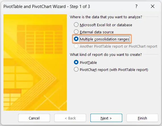
It will open the “PivotTable and PivotChart Wizard – Step 1 of 3″ dialog box.
Choose “Multiple consolidation ranges” in the first segment and PivotTable in the last. Now, click Next.
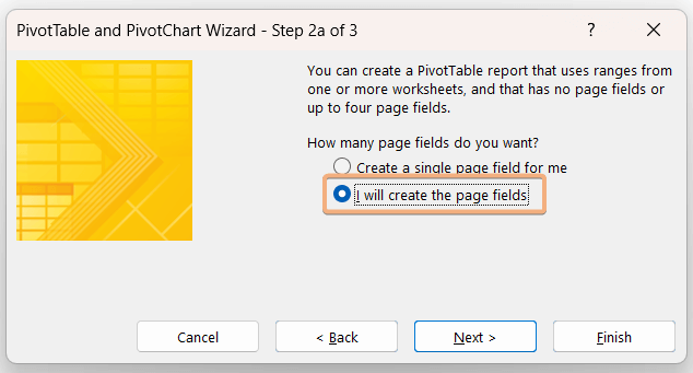
In Step 2a, select “I will create the page fields”, then click Next.

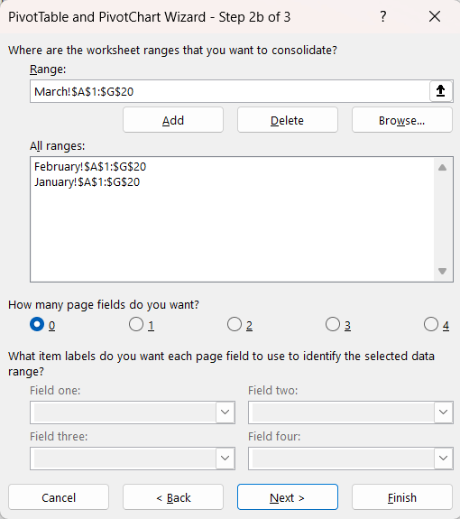
In step 2b, navigate to your first sheet, select the entire range, and select Add.
Now go to the second sheet, select the range, and hit on Add.
Navigate to the third sheet and select the range, choose Add.

Select 0 in the section “How many page fields do you want?” as we don’t want any page fields.
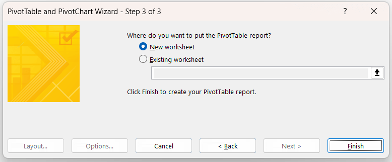
Select the location where you want to put the pivot report.
Click Finish.

Now you have created a pivot table from multiple sheets.

The values are shown in the count of value format by default. You can change the value field calculation as per your need. Then, you need to remove and add fields.

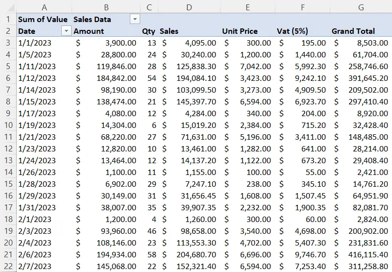
See the image. You have connected all the sheets in a pivot table. I have done some formatting to make it understandable.

Create Pivot Table from Multiple Sheets in Excel by Using Relationships Tool

When you have some data in a sheet and more details in another sheet. Then, you can create a pivot table from multiple sheets using the Relationships tool in Excel. There should be a column to relate all the sheets.

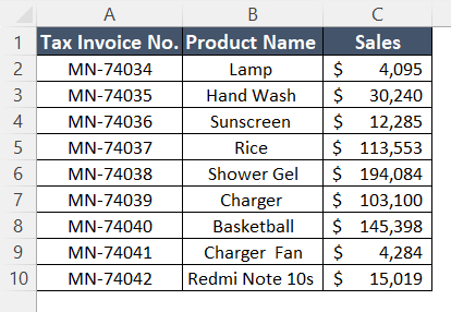
Let’s say, we have two different sets of data. In sheet 1, we have the tax invoice number with the product names and sales.

In sheet 2, we have a common column of tax invoice numbers. However, the details of that data are different from sheet 1.

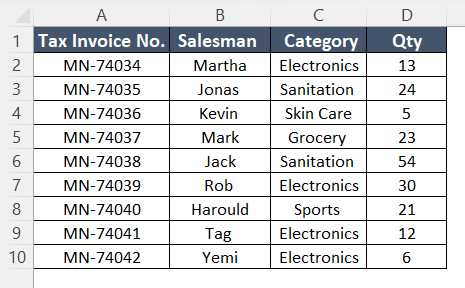
Here I will create a connection and prepare a pivot table from two sheets.

Step 1: Create Connection between Two Sheets

Now, follow these steps to create connection with Relationships Tool:

Convert data ranges into a table by pressing CTRL+T.
Go to the Data tab and choose Relationships tool from Data Tools group.
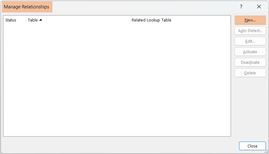
Click New command in the Manage Relationships dialog box.

Select the table name and related table to create a connection in the Create Relationship dialog box.
Choose the common column to relate.
Click OK.

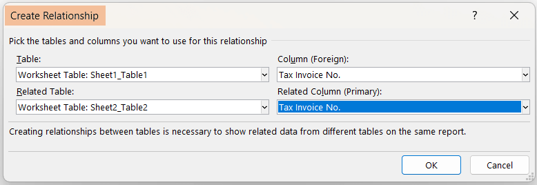
Afterward, you will see the Manage Relationships dialog box and see the connection. Now, click Close.

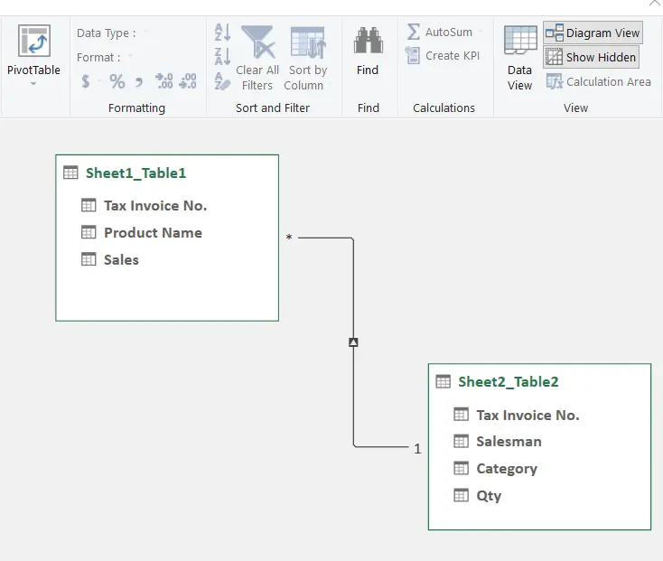
Step 2: Check whether the Relationship Created or Not

Just go to the Data Tools group and select the Power Pivot option.

This might ask your permission to enable Power Pivot.

Click on the Enable dialog box.
Select Diagram View tool under the View group in Power Pivot window.
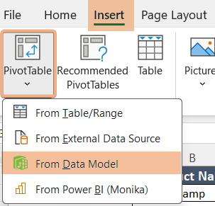
Go to Insert tab > PivotTable dropdown > From Data Model option.

Select the location and click OK.
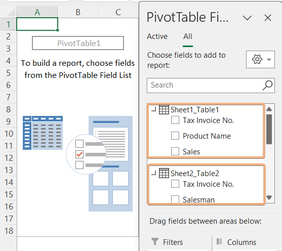
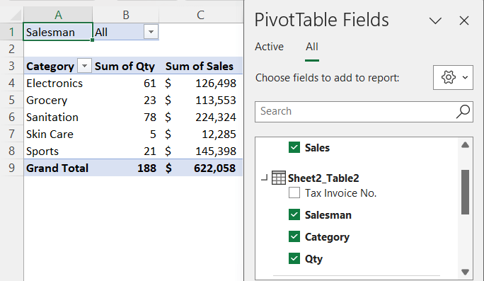
You have created a pivot table. Now, you can select the fields from different sheets.

Here from sheet 1, I have chosen the sales column and from sheet 2, I have selected the salesman, category, and quantity. I have created a pivot table from two different sheets successfully.

Create Pivot Table from Multiple Sheets in Excel Using Power Query

To create a pivot table from multiple sheets in Excel using Power Query, follow these steps:

Step 1: Import Data Into Power Query Editor

To create a pivot table from multiple sheets in Excel using Power Query, you have to convert your range into an Excel table first. Here’s how:

Select the range and click CTRL+T.
Check “My table has headers” in the Create Table dialog and hit OK.

Now go to Data tab > Get & Transform Data tool > From Table/Range option.
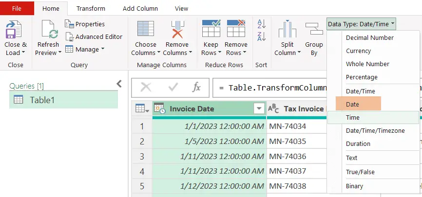
It will import your data into the Power Query Editor. Now you need to adjust the date type in the “Invoice Date” column. To do so, go to Date Type and select Date. (by default, it is Date/Time).

Step 2: Add Custom Column and Create Connections

Now, you have to add a column to track the information on different sheets. To do that:

Go to the Add Column tab and select Custom Column tool.

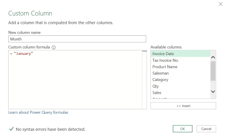
Insert a name in the new column name and input the name of the new column under the Custom column formula. Now, click OK.
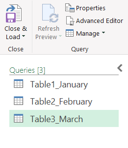
Click Close & Load. Then, repeat the same process to bring other tables to the Power Query Editor. Rename them at your convenience.
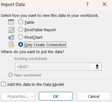
Click on the dropdown of Close & Load and select Close & Load to… the results. There will be a dialog box in the Import data dialog box. Select the Only Create Connection.

You will see this after the previous step in Queries & Connections dialog box.

Step 3: Append Data from Multiple Sheets

Now, you need to append the data together from multiple sheets. To do that, follow the instructions:

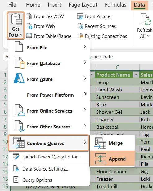
Go to Data tab > Get Data tool > Combine Queries option > Append command.
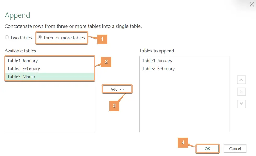
Choose three or more tables, then select the available tables, click Add, and hit OK.

Here is the appended result in Power Query Editor window.

Step 4: Load Data Into Worksheet As PivotTable Report

Now you need to close the Power Query Editor and load the data into a worksheet. To do that, follow these steps:

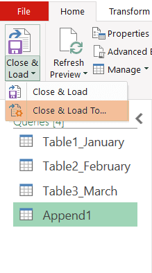
Click on the dropdown of Close & Load first.
Then, choose “Close & Load To…”.

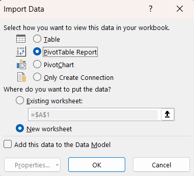
This will open the Import Data dialog box.

Now, select PivotTable Report option and choose New Worksheet to put the data.
Then, click OK.

Here, I have created a pivot table from multiple sheets by using Power Query.

Conclusion

While working on large datasets, you have to append three different sheets. From those sheets, you have to summarize and analyze datasets. When you encounter these situations, you will need to learn to create pivot tables from different sheets. In this article, I have gathered 3 methods to create a pivot table from multiple sheets. Hope this will help you out with these kind of problems.

Frequently Asked Questions

Can a Pivot Table pull from multiple sheets?

No, a Pivot Table in Excel cannot directly pull data from multiple sheets. A PivotTable is typically based on a single data source within the same worksheet or workbook. However, you can consolidate data from multiple sheets and use them as a single data source.

To consolidate data, you can consider these options:

Consolidate Data in a Single Sheet: Copy or link the data from multiple sheets into a single sheet, and then create a Pivot Table from that consolidated data.

Power Query (Get & Transform Data): In newer versions of Excel, you can use Power Query to combine data from multiple sheets, transform it, and load it into a single table for PivotTable analysis.
Use External Data Connections: Create an external data connection to another Excel workbook or an external data source to bring data from different sources into a single Pivot Table.

These methods allow you to work with data from multiple sheets in a Pivot Table, but they involve some data consolidation or data import steps.

Can a Pivot Table pull from another workbook?

Yes, a Pivot Table in Excel can pull data from another workbook. To do this:

Open the workbook containing the Pivot Table and the one you want to pull data from.
In the Pivot Table workbook, click on a cell within the Pivot Table. Go to the PivotTable Analyze tab in the Excel ribbon.

In the Data group, click on Change Data Source tool.
Now browse for the data workbook by clicking Select a Table or Range and navigate to the other workbook.
Select the data range you want to include in your Pivot Table and click OK.

The Pivot Table in your original workbook will now pull data from the selected range in the other workbook. This allows you to consolidate and analyze data from multiple sources in one Pivot Table.

How do I pull data from another sheet in the Excel Pivot Table?

To pull data from another sheet into an Excel Pivot Table, follow these steps:

Open the worksheet where you want to create the Pivot Table.

Click anywhere within the worksheet where you want the Pivot Table to be placed.
Go to the Insert tab on the Excel ribbon.
Click the dropdown of PivotTable in the Tables group and select From an external data source.

In the “PivotTable from an external source” dialog box, click on Choose Connection, then hit Browse for More.
Now, navigate to the folder that contains the data source and select the Excel sheet.
Once you’ve selected the data source, click OK to create the Pivot Table.

It will pull data from the other sheet. By following these steps, you can easily create a Pivot Table that draws its data from a different sheet in your Excel workbook, allowing you to consolidate and analyze information from multiple sources.

5/5 - (4 votes)