How to Arrange Pivot Table Columns Side by Side in Excel

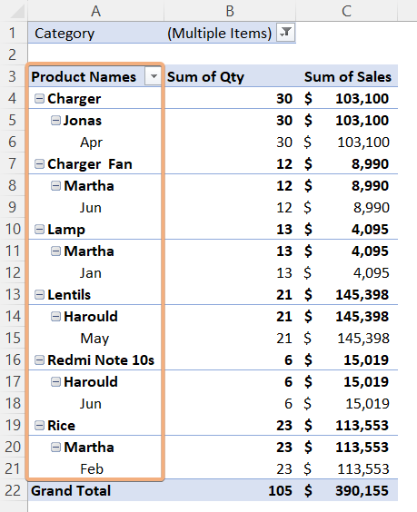
When you add multiple fields to the Rows area in a Pivot Table in Excel, by default, all the fields are displayed in the same column:

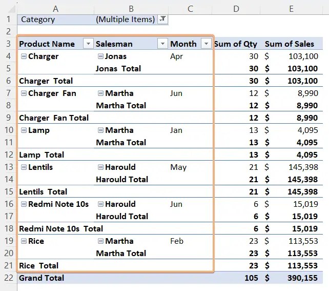
For clearer presentation of your data, you may want to organize the row labels in PivotTable columns, side by side, as follows:

In this article, we discuss two ways to change PivotTable row labels into Pivot Table columns, side by side in Excel. We will follow these quick steps:

1. Select any cell in the PivotTable to access the Design tab.
2. Click on the dropdown of Change Report Layout.
3. Select Show in Tabular Form.
4. Remove Subtotals for a cleaner look.

Keep reading for detailed instructions on how to do the above.

Adding fields to the Rows area in a Pivot Table

When we create a Pivot Table in Excel, we can add or remove fields by dragging them to the Rows or Columns areas in the PivotTable Fields pane.

In the example above, you will see that we have added Product Name, Salesman, and Month to the Rows area.

In the resulting Pivot Table, we can see the listed row labels in the same column by default.

Let’s see how we can show these fields as separate Pivot Table columns, side by side, to make things a bit clearer.

Method 1: Change Report Layout to Set up Pivot Table Columns Side by Side

We can display the columns side by side, by changing the report layout to tabular form:

1. Click anywhere in the Pivot Table.
2. Then, go to the Design tab.
3. Next, click the dropdown of Change Report Layout.
4. Now, choose Show in Tabular Form option.
   

This will change your Pivot Table layout to tabular form, and show the fields in separate Pivot Table columns, side by side. The fields Product Name, Salesman and Month now each have their own column:

Remove the Totals from the Pivot Table

You will notice subtotals all throughout the Pivot Table, after arranging the columns to be side by side. This looks rather messy, so let’s get rid of them.

To do so, follow the instructions below:

1. Right-click the header cell from which column you want to remove totals in the Pivot Table.
2. Then, select Subtotal “xxx” from the Context Menu, with “xxx” being the heading of the field that you want to remove the totals for.
   
3. Repeat the same process for the other columns.

Removing the subtotals gives us a much cleaner look, when showing Pivot Table columns side by side.

Method 2: Arrange Pivot Table Columns Side by Side Using PivotTable Options

Another way to prevent the PivotTable fields from being in the same column and be displayed across multiple columns instead, you can use PivotTable Options. Here’s how:

1. 1. Right-click any cell in the Pivot Table.
   2. Then, choose PivotTable Options from the Context Menu.
      
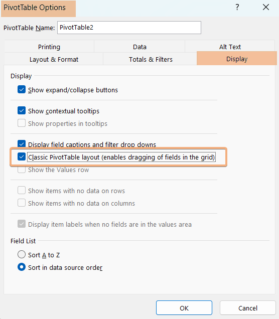
   3. Next, go to Display tab in the PivotTable Options dialog box.
   4. Now, check on the Classic PivotTable layout and click OK.
      

As a result, this will update your Pivot Table columns side by side.

Remember to remove subtotals, as explained under Method 1 above.

Frequently Asked Questions

How do I order columns in a Pivot Table?

To order columns in a Pivot Table in Excel, you can follow these steps:

1. Click anywhere within the Pivot Table to select it.
2. In the PivotTable Fields, rearrange your fields to control the order.
3. To change the order of columns, you can drag a field from the Columns area and drop it into a different position within the Columns area.
4. You can also use the Column Labels area to rearrange fields to change the order of columns in your Pivot Table.

By reordering the fields within the Columns and Column Labels areas of your Pivot Table, you can control the sequence and arrangement of columns to best suit your data analysis and presentation needs.

How do I group multiple columns in a Pivot Table?

To group multiple columns in a Pivot Table in Excel, follow these steps:

1. Click anywhere within the Pivot Table to select it.
2. In the PivotTable Fields, hold down the CTRL key to select multiple columns to group.
3. Right-click on one of the selected columns, and then choose Group from the context menu.
   Excel will create a new grouped field in your Pivot Table. You can then further customize the grouping by right-clicking the grouped field, choosing Group again, and specifying the grouping criteria, such as date ranges or custom categories.

Grouping multiple columns in a Pivot Table allows you to create a more organized and concise data summary for analysis and reporting.