4 Cases of Excel Vlookup with Column Index Number from Another Sheet
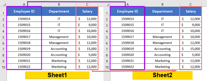
Sheet1 has a datasheet of 3 columns. Which are Employee ID, Department, & Salary. Then, Sheet2 also has a datasheet of 3 columns. The columns are Employee ID, Department, and Salary. Here, I will show you how to extract the Salary amount from Sheet1 to Sheet2 based on the Employee IDs.
What is Column Index Number in Vlookup?
Column Index Number is referred to as Col_index_num in Excel vlookup functions. It indicates the relative position number of a column in a certain range. You may want to specify the column index number in your vlookup formula to refer to a column that you want to extract from the output.
For example, we want to use the range A2:D10 as the table array. In this range, there are 4 columns available. They are column A (range A2:A10), column B (range B2:B10), column C (range C2:C10), column D (range D2:D10).
Now, when we use 1 as the column index number, it refers to column A (range A2:A10). Similarly, column index number 2 refers to column B (range B2:B10), 3 refers to column C (range C2:C10), and 4 refers to column D (range D2:D10).
Vlookup Using Column Index Number from Another Sheet
Conducting a VLOOKUP using column index numbers from another sheet in Excel is a powerful technique that enhances data retrieval and analysis. This approach allows you to reference data across sheets by column index, offering flexibility and efficiency in managing large datasets. In this guide, we’ll explore how to leverage VLOOKUP with column index numbers, providing you with a dynamic method to extract and analyze information for 4 different cases.
Case 1: Within the Same Workbook
In Sheet2, I’ve 3 columns, Employee ID, Department, and Salary. The Employee ID & Department columns are filled up. But the Salary column is completely blank. In Sheet1, there are 3 columns two, Employee ID, Employee Name, & Salary.
Now, I’m going to extract the salaries in the Salary column of Sheet2 based on the Employee IDs from Sheet1. For this purpose, I’m going to use the VLOOKUP function.
Syntax
=VLOOKUP (lookup_value, table_array, column_index_num, [range_lookup])Array Formula
=VLOOKUP(A2:A10,Sheet1!$A$2:$C$10,3,FALSE)Formula Explanation
- The range A2:A10 is an array of lookup values.
- $A$2:$C$10 is the table array. This is basically the range of the cells where the formula will look for the results. ‘Sheet1!’ is used before the table array range to mean that this table array range is located in Sheet1. If you don’t mention ‘Sheet1’ before the table array range, it will look for the results in the same worksheet.
- 3 is the column index number. This means the output is located in the 3rd column of the table array range. The 3rd column in the table array range $A$2:$C$10 is column C. Which is the Salary column.
- Finally FALSE means the VLOOKUP function must look for the exact match between the lookup value array A2:A10 and the table array range $A$2:$C$10.
Excel for Microsoft 365: Insert the formula in cell C2 and press ENTER. As it is an array formula, it will copy down itself from cell C2 to C10 automatically.
For Excel 2019 and Previous Versions: Press CTRL + SHIFT + ENTER to insert the formula into a cell instead of just pressing the ENTER button.
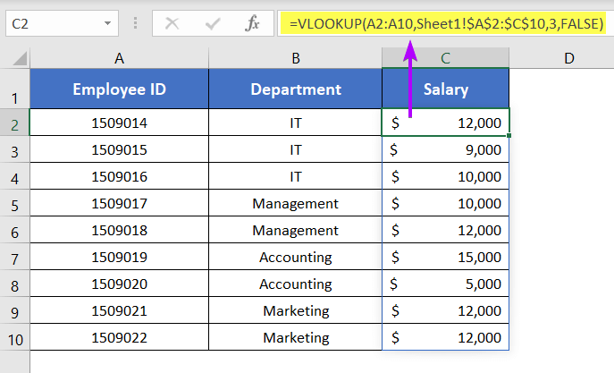
The previous one is an array formula. But if you don’t like array formulas, here’s the regular form of the previous formula for you.
Regular Formula
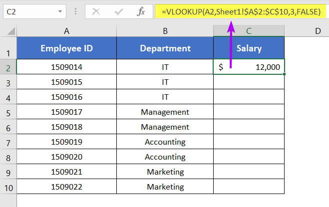
=VLOOKUP(A2,Sheet1!$A$2:$C$10,3,FALSE)To use VLOOKUP for column index number from another sheet, follow these steps below:
- Select an empty cell.
- Insert the formula:=VLOOKUP(A2,Sheet1!$A$2:$C$10,3,FALSE)
- Then, drag down the formula with Fill Handle.
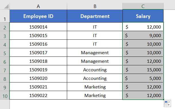
After copying down the formula, you will get the corresponding salaries against the Employee IDs in the Salary column.
Case 2: From Another Workbook
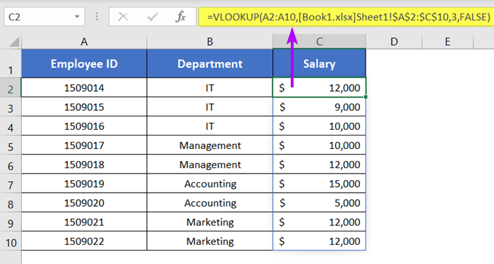
In this case, Sheet1 is located in the ‘Book1.xlsx’ workbook. Sheet2 is located in the ‘Book2.xlsx’ workbook. To vlookup for salaries from ‘Sheet1, Book1.xlsx’ to ‘Sheet2,Book2.xlsx’ use the following formula using the VLOOKUP function.
Syntax
=VLOOKUP (lookup_value, table_array, column_index_num, [range_lookup])Array Formula
=VLOOKUP(A2:A10,[Book1.xlsx]Sheet1!$A$2:$C$10,3,FALSE)Formula Explanation
- $A$2:$C$10 is the table array range.
- [Book1.xlsx]Sheet1!$A$2:$C$10 means the table array range $A$2:$C$10 is located in Sheet1 in the workbook ‘Book1.xlsx’. If you don’t mention the workbook name, the VLOOKUP function will consider the table array range is located in the same workbook.
Click_here to read how this formula actually works.
Excel for Microsoft 365: Insert the formula in cell C2 and press ENTER. As it is an array formula, it will copy down itself from cell C2 to C10 automatically.
For Excel 2019 and Previous Versions: Press CTRL + SHIFT + ENTER to insert the formula into a cell instead of just pressing the ENTER button.
The previous one is an array formula. But if you don’t like array formulas, here’s the regular form of the previous formula for you.
Regular Formula
=VLOOKUP(A2,[Book1.xlsx]Sheet1!$A$2:$C$10,3,FALSE)Now, apply VLOOKUP to use column index number from another workbook, go through these steps below:
- Select a blank cell.
- Write the formula: =VLOOKUP(A2,[Book1.xlsx]Sheet1!$A$2:$C$10,3,FALSE)
- Then, copy down the formula to the rest of the cell by dragging down the Fill Handle icon.
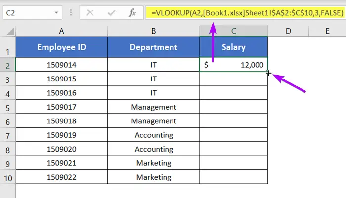
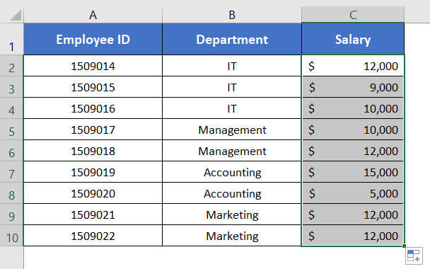
After applying the formula all over the range C2:C10, in you get the corresponding salaries in the Salary column. Have a look.
Case 3: From Multiple Sheets of the Same Workbook
In Sheet3 of the workbook ‘Book1.xlsx’, employee salaries are recorded against the Employee IDs from 1509014 to 1509020. In Sheet4 of the workbook ‘Book1.xlsx’, employee salaries are recorded against the Employee IDs from 1509021 to 1509027.
Now, I will show you how to vlookup from multiple sheets using the Column Index Number. I will combine these two data tables to create a complete list of salaries for Employee ID 1509014 to 1509027.

Basic Formula Syntax
=IFERROR(VLOOKUP(…), IFERROR(VLOOKUP(…), …, "No Data"))Regular Formula
=IFERROR(VLOOKUP(A2, Sheet3!$A$2:$C$8, 3,FALSE), IFERROR(VLOOKUP(A2,Sheet4!$A$2:$C$8,3, FALSE), "No Data"))Formula Explanation
The VLOOKUP function uses A2 to look up vertically through $A$2:$C$8 in both Sheet3 and Sheet4. Then it returns the 3rd column of the range $A$2:$C$8 which is column C. The argument FALSE tells the VLOOKUP function that the matching between the lookup value A2 and the table array range $A$2:$C$8 has to be exact.
Reminder: Make sure that the lookup column is the first column of the table array. Here, the lookup column is A2:A10 which is the first column of the table array $A$2:$C$10.
The IFERROR function returns the extracted value by the VLOOKUP function. But if the VLOOKUP function cannot return any value, the IFERROR function returns the message ‘No Data’.
To vlookup among multiple sheets, I’m going to use a formula with the IFERROR and VLOOKUP functions. Now, follow the steps below:
- Select cell C2.
- Copy and paste the formula in the selected cell:=IFERROR(VLOOKUP(A2, Sheet3!$A$2:$C$8, 3,FALSE), IFERROR(VLOOKUP(A2,Sheet4!$A$2:$C$8,3, FALSE), “No Data”))
- Then, use Fill Handle icon to drag down the formula to the column.
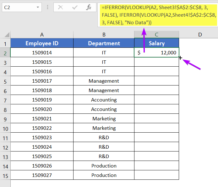
After copying down the vlookup formula, you will get the complete list of salaries for Employee IDs 1509014 to 1509027 in the Salary column.
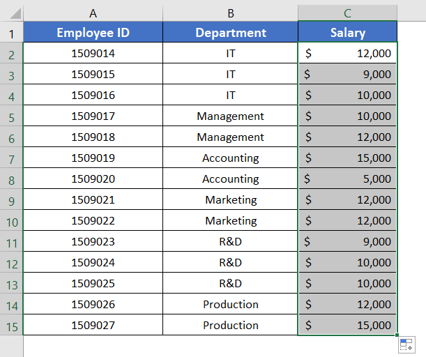
If you are looking for the array formula version of the above vlookup formula, here you go.
Array Formula
=IFERROR(VLOOKUP(A2:A15, Sheet3!$A$2:$C$8, 3,FALSE), IFERROR(VLOOKUP(A2:A15,Sheet4!$A$2:$C$8,3, FALSE), "No Data"))Excel for Microsoft 365: Insert the formula in cell C2 and press ENTER. As it is an array formula, it will copy down itself from cell C2 to C10 automatically.
For Excel 2019 and Previous Versions: Press CTRL + SHIFT + ENTER to insert the formula into a cell instead of just pressing the ENTER button.
Case 4: From Multiple Sheets of a Different Workbook
In Sheet3 of the workbook ‘Book1.xlsx’, employee salaries are recorded against the Employee IDs from 1509014 to 1509020. In Sheet4 of the workbook ‘Book1.xlsx’, employee salaries are recorded against the Employee IDs from 1509021 to 1509027.
Now, I want to extract the salaries against the Employee IDs from 1509014 to 1509027. I want to merge two salary lists from Sheet3 & Sheet4 of ‘Book1.xlsx’ and put them into Sheet5 of ‘Book2.xlsx’.

For this purpose, I’m using the following formula having the IFERROR and the VLOOKUP functions.
Basic Formula Syntax
IFERROR(VLOOKUP(…), IFERROR(VLOOKUP(…), …, "No Data"))Regular Formula
=IFERROR(VLOOKUP(A2, [Book1.xlsx]Sheet3!$A$2:$C$8, 3,FALSE), IFERROR(VLOOKUP(A2,[Book1.xlsx]Sheet4!$A$2:$C$8,3, FALSE), "No Data"))Formula Explanation
The VLOOKUP function uses A2 to look up vertically through $A$2:$C$8 in both Sheet3 & Sheet4 of ‘Book1.xlsx’. Then, it returns the 3rd column of the range $A$2:$C$8 of ‘Book1.xlsx’ which is column C. The argument FALSE tells the VLOOKUP function that the matching between the lookup value A2 and the table array range $A$2:$C$8 has to be exact.
Reminder: Make sure that the lookup column is the first column of the table array. Here, the lookup column is A2:A10 which is the first column of the table array $A$2:$C$10.
The IFERROR function returns the extracted value by the VLOOKUP function. But if the VLOOKUP function cannot return any value, the IFERROR function returns the message ‘No Data’.
Follow the steps to use column index number from another workbook:
- Select cell C2.
- Insert the formula: =IFERROR(VLOOKUP(A2, [Book1.xlsx]Sheet3!$A$2:$C$8, 3,FALSE), IFERROR(VLOOKUP(A2,[Book1.xlsx]Sheet4!$A$2:$C$8,3, FALSE), “No Data”))
- Then, copy down the formula up to cell C15 with Fill Handle.
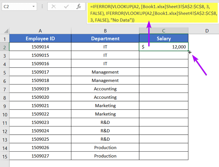
After copying down the vlookup formula, you will get the complete list of salaries for Employee IDs 1509014 to 1509027 in the Salary column.
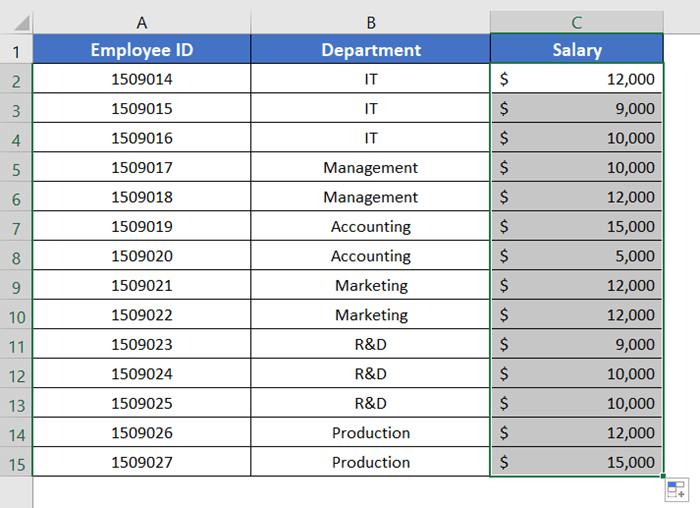
If you are looking for the array formula version of the above vlookup formula, here you go.
Array Formula
=IFERROR(VLOOKUP(A2:A15, [Book1.xlsx]Sheet3!$A$2:$C$8, 3,FALSE), IFERROR(VLOOKUP(A2:A15[Book1.xlsx]Sheet4!$A$2:$C$8,3, FALSE), "No Data"))Excel for Microsoft 365: Insert the formula in cell C2 and press ENTER. As it is an array formula, it will copy down itself from cell C2 to C10 automatically.
For Excel 2019 and Previous Versions: Press CTRL + SHIFT + ENTER to insert the formula into a cell instead of just pressing the ENTER button.
Conclusion
I tried to help you to vlookup from another sheet in Excel using a column index number. I expect you’ve found this article useful. You can read more articles relating to Excel from the Blog page of our website. Have a fantastic workday!
Frequently Asked Questions
How to use column index number in Excel?
To use column index numbers in Excel, employ the VLOOKUP function. Specify the column index number as the second argument in the VLOOKUP formula, indicating the column from which to retrieve data. For example: =VLOOKUP(lookup_value, table_array, column_index_number, [range_lookup])
In this formula, ‘column_index_number’ represents the position of the desired data column within the ‘table_array.’ The lookup result will be retrieved from the specified column. This technique proves invaluable for dynamic data retrieval and analysis, allowing users to efficiently reference information across sheets or tables based on column index numbers.
How do I give a column index number in VLOOKUP?
To assign a column index number in VLOOKUP, simply include it as the third argument in the formula. The syntax is as follows: =VLOOKUP(lookup_value, table_array, column_index_number, [range_lookup])
Specify the ‘column_index_number’ parameter to indicate the position of the desired data column within the ‘table_array.’ Excel will then retrieve information from the specified column based on the provided index number. This streamlined approach enhances data lookup processes and is particularly useful for referencing and analyzing information across different columns within your Excel workbook.
How do I use VLOOKUP to get value from another sheet?
To use VLOOKUP to get a value from another sheet in Excel, include the sheet name and cell reference as part of the ‘table_array’ argument. The syntax is as follows: =VLOOKUP(lookup_value, ‘Sheet2’!$A$1:$B$10, 2, FALSE)
In this formula, replace ‘Sheet2’ with the actual name of the sheet containing the data. The ‘table_array’ now references cells on another sheet, and the VLOOKUP function will retrieve the value based on the specified lookup criteria. This technique streamlines data retrieval and analysis, enabling efficient cross-sheet referencing in your Excel workbooks.
