How to Sort Pivot Table by Sum in Excel [2 Cases]

By sorting the Pivot Table by sum in Excel in descending or ascending order, users can quickly identify the highest or lowest contributing factors within their dataset. This capability is essential for gaining insights into trends, patterns, and key metrics, making it a valuable asset for data analysis and decision-making. In this article, I will discuss 2 types of Pivot Table sorting by sum in Excel. Let’s explore the guidelines.

Table of Contents

How to Sort Vertically by Sum in Excel Pivot Table

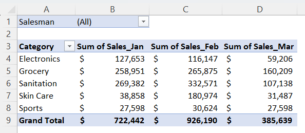
In this Pivot Table, I have a summarized sales report. Here are 3 months of sales value with category. Now, I will sort the sum value horizontally and vertically.

Step 1: Add a Calculated Field

To sort the Pivot Table by sum horizontally in Excel, follow these steps:

Select any cell inside the Pivot Table and go to PivotTable Analyze tab.
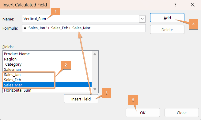
Click on the dropdown of Fields, Items, & Sets under the Calculations group and hit Calculated Field.
First, enter a name in the Name box in the Insert Calculate Field dialog box.

Then, choose and click from the Fields you want to insert in the formula box and hit Insert Field.
Next, click Add and hit OK.

Here, I have got a new column with the summation of the sales data of previous months. Now, I will sort them vertically.

Step 2: Use Pivot Table Sort by Sum

To sort vertically, follow the steps:

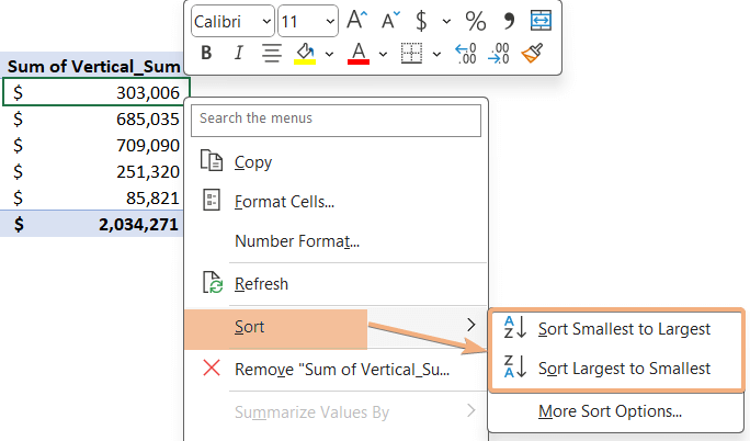
Select a cell in the Pivot Table and right-click on that.
Now, click on Sort.

Choose from Sort Smallest to Largest and Sort Largest to Smallest.

Here, I chose Sort Smallest to Largest.

How to Sort Horizontally by Sum in Excel Pivot Table

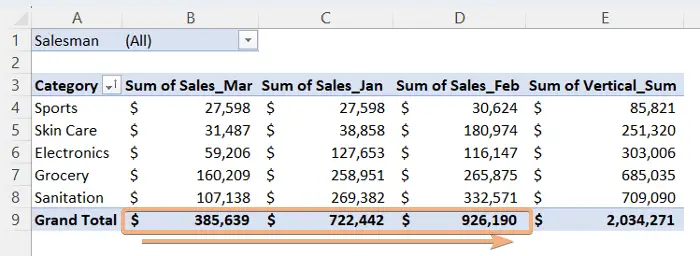
To sort the Pivot Table by sum horizontally in Excel, I will sort the Grand Total row. In this row, the summation of each column is there.
Now, follow the instructions below:

Select a cell in the Grand Total row and right-click on that.
Choose sort options from Sort.
Here I have selected Sort Smallest to Largest.

See the screenshot. I have sorted the Pivot Table by sum horizontally in Excel.

Conclusion

In conclusion, sorting a Pivot Table by sum in Excel is a powerful feature that allows users to arrange data based on aggregated values. In this article, I have added 2 types of sorting Pivot Table by sum. Additionally, I have included a calculated column in the Pivot Table before sorting by sum vertically. So, I hope, this is a complete guide to sort Pivot Table by sum in Excel.

Frequently Asked Questions

How do you sort a Pivot Table by sum amount?

To sort a Pivot Table by the sum amount, follow these steps:

Locate the header of the column containing the sum amounts in your Pivot Table.

Right-click on the header cell of the sum amount column.
In the context menu, select either Sort Largest to Smallest or Sort Smallest to Largest, depending on your preference.

This action will rearrange the rows in the Pivot Table based on the sum amounts, placing the largest or smallest values at the top. Sorting by sum amount is useful for quickly identifying the most significant or least significant values in your data.

How do I filter sums in a Pivot Table?

To filter sums in a Pivot Table, you can use the Value Filters option. Here’s how:

Locate the drop-down arrow next to the header of the column containing the sum values in your Pivot Table.
Hover over the drop-down arrow, and in the menu that appears, select Value Filters.

Choose the type of filter you want, such as Greater Than, Less Than, Equals, etc.
Enter the specific value you want to use as a filter criterion and click OK.

This will filter the Pivot Table to display only the rows where the sum values meet the specified criteria. Filtering sums is helpful when you want to focus on specific ranges or subsets of data based on the aggregated values in your Pivot Table.

How do I fix sort in a PivotTable?

To fix sorting issues in a Pivot Table, you can follow these steps:

Check for Blank Cells: Ensure that there are no blank cells in the column you are trying to sort. Blank cells can disrupt the sorting process.
Remove Filters: Remove any filters applied to the Pivot Table. Filters can interfere with sorting.

Refresh the PivotTable: Refresh the PivotTable to make sure it reflects the latest changes in the underlying data.
Verify Data Format: Check the format of the data in the column. If it contains a mix of text and numeric values, Excel may not sort it correctly. Ensure consistent formatting.
Reapply Sorting: If the issue persists, try reapplying the sorting. Right-click on the column header, choose Sort and select the appropriate sorting option.

Check for Grouping: If the PivotTable includes grouped items, ungroup them before sorting to avoid unexpected results.
Reset Custom Sorting: If you’ve applied custom sorting, reset it to default settings and try sorting again.
Clear Manual Sorting: If you have manually rearranged items, clear any manual sorting by choosing More Sort Options and selecting Sort automatically.

By following these steps, you can troubleshoot and fix sorting issues in your Pivot Table. Regularly updating and refreshing the Pivot Table, along with maintaining consistent data formatting, will help ensure accurate and reliable sorting.

Rate this post