6 Methods to Paste Range Names in Excel

While dealing with large spreadsheets, it becomes necessary to name the ranges in Excel first. Additionally, you can track and organize your data in an Excel sheet. Sometimes you have to quickly paste the range names in another location to make your work fast. In this article, you will learn what is named range and the methods to paste range names in Excel in 6 different ways.

Table of Contents

What is Named Range in Excel?

The named range is a useful way to track your data especially while applying a formula in Excel. In this case, you have to select a range and assign a name. Then, if you want to apply a formula, or make any change, you don’t have to change in all cells manually. If you make a change, Excel will update it over the entire range.

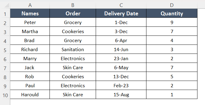
Here is a dataset of different ranges.

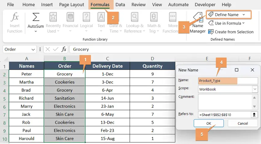
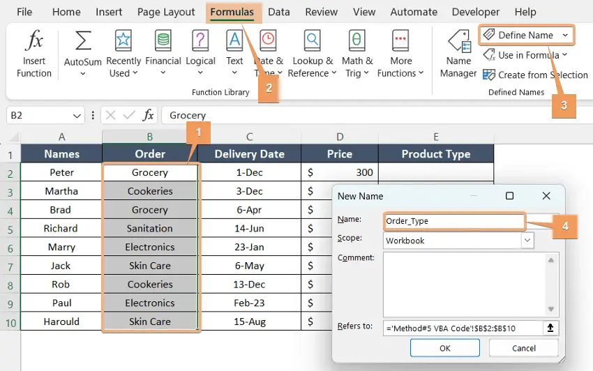
If you want to name the range B2:B10, follow the instructions below:

Select the Range B2:B10.

Then, go to Formulas.
Next, click on Define Names.
Afterward, the New Name window will appear.
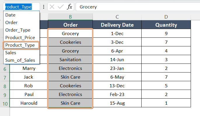
Now, enter a name for your range and click OK. Now, if you click on the dropdown of the Name Box, you will see the name you applied to a range.

How to Paste Range Names inside a Formula in Excel

To paste range names in Excel, you can follow the below-mentioned instructions.

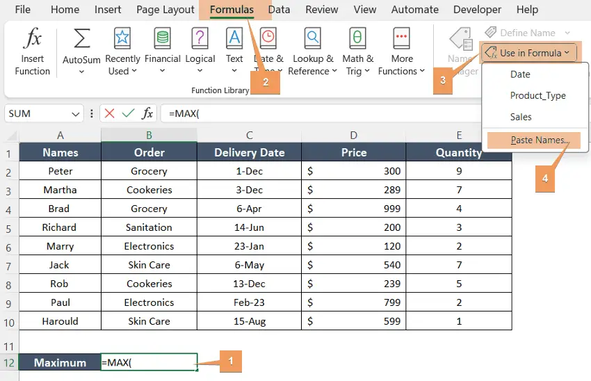
Firstly, select cell B12 and write the function.
Here I have used MAX to apply formulas.

Then, go to the Formulas tab.
Next, click the dropdown of Use in Formula and select Paste Names.
After that, the Paste Name dialog box will appear.
Now, select Sales and click OK.
Finally, you have got the maximum price by using the paste name of the range.

How to Paste Range Names in Excel Using Paste Name Options

If you need to paste a range of data, you can simply use the Paste Names option. Follow the steps to paste range names in Excel:

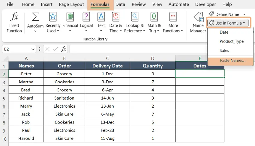
At first, insert a column to paste the range of data.
Then, select cell E2. Next, go to the Formulas tab and click the dropdown on the Use in Formula. Now, choose Paste Names.

Select Date in the Paste Name dialog box and click OK. After that, you will see this interface.
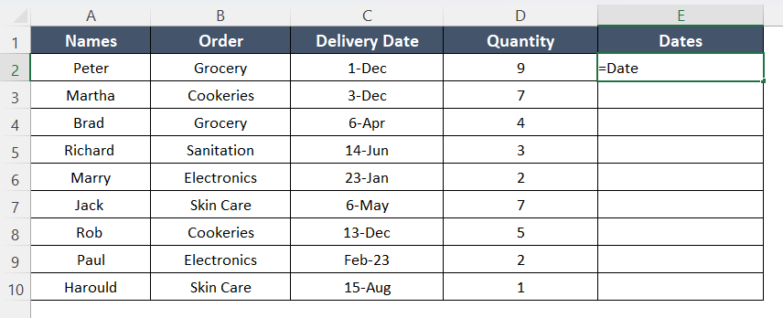Now, press ENTER. You have pasted the range of dates successfully. Keep in mind to format the cells if you are pasting the dates.

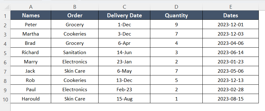
How to Paste Range Names in Excel Applying the Paste List Option

If you want to paste the list of these ranges, then you just choose the option Paste List from Use in Formula dropdown.

Here’s how to do it in easy steps:

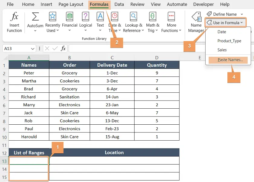
Select cell A13.
Now, go to Formulas. Click the dropdown in Use in Formula. Choose Paste Names.

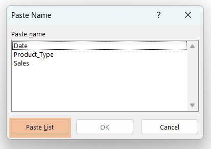
Now, select Paste List on the Paste Name dialog box. Don’t merge any cells. Otherwise, it won’t show the desired output. Now you can see the list of ranges with the location of the sheets.

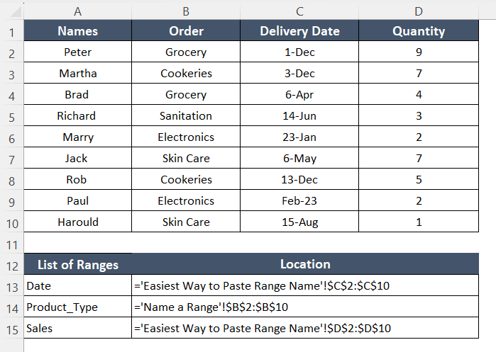
How to Paste Range Names in Excel Using Shortcut Keys

In Office 365, when you include a range within a formula, it should be automatically replaced with its corresponding range name if one exists. However, if this automatic transition from a range to a range name does not occur, you can manually do it by following the steps below:

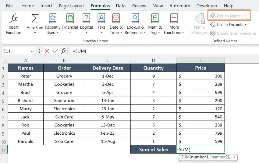
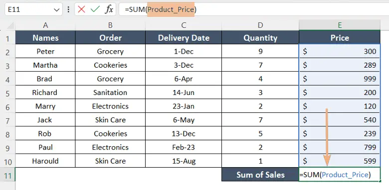
Select cell E11 and enter the function.

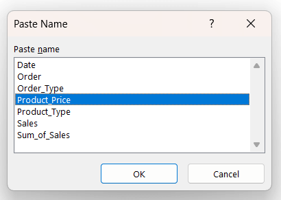
You can see Define Name has been greyed out. To paste the range name, press the F3 key to bring the list of all named ranges.
Select your required range name from the list and hit OK.
Your intended range within your formula should be replaced with the corresponding range name instantly.

Just hit ENTER to proceed. You have successfully replaced your range with a named range inside your formula.

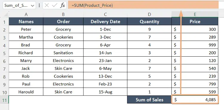
How to Paste Range Names in Excel Using Formula Assistance

Another way to paste range names in Excel is formula assistance. The steps are below:

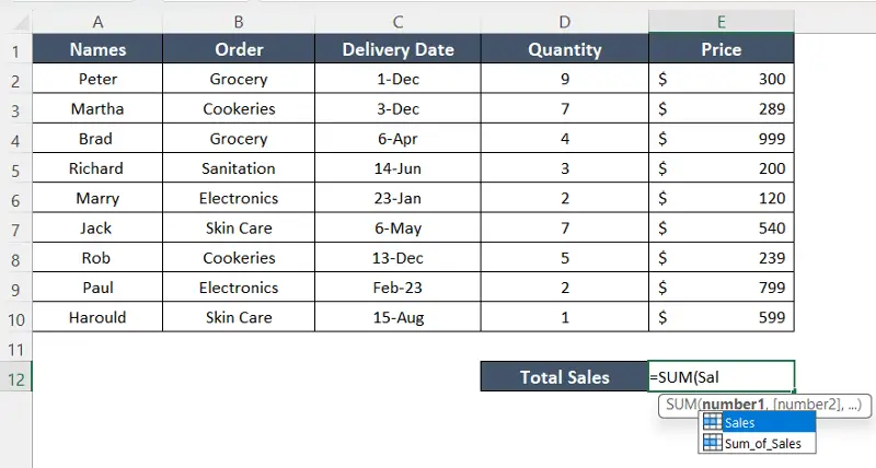
Select cell E12.

Apply a formula. Here, I have inserted the SUM function.
Start to type the range name and there will be a list of suggestions. Now, double-click on the range name and press ENTER.
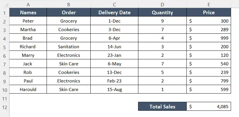
Here is the output it shows after using formula assistance to paste range names.

How to Paste Range Names in Excel Using VBA Code

You can use a VBA code as an alternate method of pasting range names in Excel.

Now, go through the directions below:

Select a range to name the range. Then go to Formulas. Click on Define Name. Now, insert a name in the New Name dialog box and click OK.

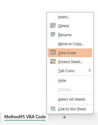
Then, go to the sheet’s name and right-click on that. Now, select View Code to open the Visual Basic Editor.
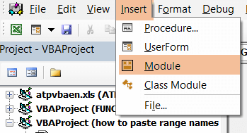
Click on Insert > Module in Visual Basic Editor.

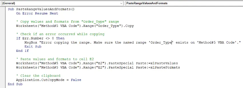
Copy the code below and paste it.
Make sure, you have edited the sheet’s name and range name according to your worksheet.

Sub PasteRangeValuesAndFormats()
    On Error Resume Next
    ' Copy values and formats from "Order_Type" range
    Worksheets("Method#5 VBA Code").Range("Order_Type").Copy 
    ' Check if an error occurred while copying
    If Err.Number <> 0 Then
        MsgBox "Error copying the range. Make sure the named range 'Order_Type' exists on 'Method#5 VBA Code'."
        Exit Sub
    End If
    ' Paste values and formats to cell E2
    Worksheets("Method#5 VBA Code").Range("E2").PasteSpecial Paste:=xlPasteValues
    Worksheets("Method#5 VBA Code").Range("E2").PasteSpecial Paste:=xlPasteFormats
    ' Clear the clipboard
    Application.CutCopyMode = False
End Sub

Copy and Paste the VBA code to paste range names in Excel

Now, return to the worksheet. Then, press ALT+F8 to open the Macros dialog box and click Run. Now, look at the image. I have pasted the range names in column E successfully.

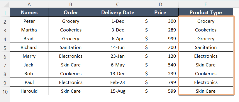
Keyboard Shortcuts Related to Range Names in Excel

While working with pasting range names, you have to use some shortcuts in some cases.

To obtain the list of range names, press F3.
To create a New Name while using Name Manager, press CTRL+F3.
To create a range name from cell selection, press CTRL+SHIFT+F3.

Conclusion

To sum up, I have described 6 methods to paste range names in Excel. All methods include the Define Name and Use in Formula commands under the Formulas tab. If you have no idea what the named range is and how to name ranges in Excel, I have also added the guide to name ranges for your reference. Now, your work will be easier to apply formulas in a range of cells by pasting the range names. You can also solve the issues regarding this problem by following this guide.

Frequently Asked Questions

What is Paste Special in Excel?

Paste Special in Excel is a feature that allows users to control and customize the way data is pasted from the clipboard into a selected range. It provides various options beyond the standard paste, enabling users to selectively paste specific aspects of the copied data.

Can you paste cells without the formulas?

To paste cells without formulas in Excel, use the Paste Special feature. Here’s how:

Copy the cells or range that you want to paste.
Choose the destination range where you want to paste the content.
Right-click on the selected destination range.

From the context menu, choose Paste Special.
In the Paste Special dialog box, select the Values option.
Click the OK button to paste only the values into the selected range.

This method pastes the content without including the underlying formulas. It’s a useful technique when you want to retain the data without transferring the calculations from the source range.

How do you paste in Excel without formulas?

To paste in Excel without formulas and only paste the values, follow these steps:

Copy the data that you want to paste.

Select the destination range where you want to paste the values.
Right-click on the selected destination range.
Choose Paste Special from the context menu.

In the Paste Special dialog box, choose the Values option.
Click the OK button to paste only the values into the selected range.

This method pastes the content without bringing along the underlying formulas. It is useful when you want to retain the data but not the calculations from the source range.

Rate this post