How to Use NOT Function in Excel [2 Examples]

In the realm of Excel functions, the NOT function stands out as a powerful tool for logical operations. While its name might suggest a negation, its actual application extends beyond mere negation. In this article, we will delve into the intricacies of the NOT function, exploring its syntax, arguments, and outputs, and providing real-world examples to illustrate its usage effectively.

Table of Contents

What Does the Excel NOT Function Do?

The NOT function in Excel serves to evaluate whether a given logical statement is FALSE. Essentially, it reverses the logical value of its argument. If the argument is TRUE, NOT returns FALSE; if the argument is FALSE, NOT returns TRUE. This simple yet versatile function finds application in various scenarios, from data validation to conditional formatting.

What is the Syntax of the Excel NOT Function?

The syntax of the NOT function in Excel is straightforward:

=NOT(logical)

Here, logical represents any expression or value that can be evaluated as either TRUE or FALSE.

What are the Arguments of the Excel NOT Function?

The Excel NOT function accepts only one argument:

logical: This is the value or expression that you want to evaluate. It can be a cell reference, formula, or logical expression.

What is the Output of the Excel NOT Function?

The output of the Excel NOT function is a logical value:

TRUE: If the logical argument is FALSE.
FALSE: If the logical argument is TRUE.

2 Examples of Using the NOT Function in Excel

Let’s explore some practical examples to grasp the application of the NOT function:

Example 1: Checking if a Value is Not Equal to a Specific Criteria

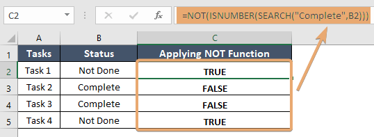
Suppose you have a dataset in column B, and you want to check if any cell does not contain the value “Complete.” You can use the NOT function in combination with the ISNUMBER and SEARCH functions:

=NOT(ISNUMBER(SEARCH("Complete",B2)))

This formula returns TRUE if the cell does not contain “Complete” and FALSE if it does.

Example 2: Verifying if a Number is Not Equal to Zero

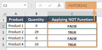
Suppose you have a set of numbers in column B, and you want to identify which ones are not equal to zero:

=NOT(B2=0)

This formula will return TRUE for cells in column B that contain values other than zero.

Things to Remember

The NOT function reverses the logical value of its argument.
It returns TRUE if the argument is FALSE, and FALSE if the argument is TRUE.

The logical argument can be any expression or value that evaluates to TRUE or FALSE.
Utilize the NOT function in combination with other Excel functions for enhanced data analysis and manipulation.

Conclusion

In conclusion, the Excel NOT function is a valuable tool for logical operations, offering versatility and efficiency in data analysis tasks. By understanding its syntax, arguments, and practical examples, you can leverage its capabilities to streamline your Excel workflows and make informed decisions based on your data.

Frequently Asked Questions

Can I use the NOT function with multiple conditions?

Yes, you can combine the NOT function with other logical functions like AND and OR to evaluate multiple conditions simultaneously.

Does the NOT function work with text values?

Yes, you can use the NOT function with text values, where the empty text (“”) evaluates to FALSE and any non-empty text evaluates to TRUE.

Is there a limit to the number of arguments the NOT function can accept?

No, the NOT function accepts only one argument, which can be any valid logical expression or value.

Can I nest the NOT function within other functions?

Yes, you can nest the NOT function within other functions to create more complex logical expressions and formulas in Excel.

Rate this post