3 Methods to Lock Pivot Table Column Width in Excel

To lock the Pivot Table column width, follow the steps:

1. Select any cell within the Pivot Table.
2. Navigate to the PivotTable Analyze tab > Options under the PivotTable group.
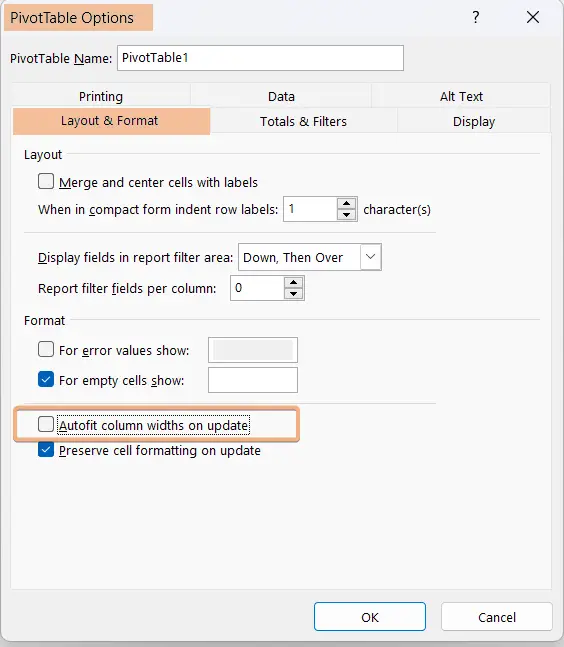
3. Go to the Layout & Format tab in the PivotTable Options dialog box.
4. Now, uncheck on “Autofit column widths on update” and click OK.

After going through all the steps, this won’t update the column widths while entering new data into the Pivot Table.

Lock Pivot Table Column Width by Turning off Autofit Column Widths

I have a dataset of sales reports in Pivot Table to lock the Pivot Table Column Width in Excel.

While inserting a Pivot Table, it adjusts the column width automatically. So, turn off autofit column width to lock the Pivot Table column width in Excel. Now, follow these steps to do that:

1. Click on a cell in the Pivot Table.
2. Then, go to PivotTable Analyze tab > Options under the PivotTable group.
3. Next, go to Layout & Format in the PivotTable Options dialog box.
4. Uncheck “Autofit column widths on update” and click OK.
   

Now, I will add any other field to the Pivot Table from PivotTable Fields. So, it won’t update the Pivot Table column width in Excel.

Lock Pivot Table Column Width Using Protect Sheet Option

To lock the Pivot Table column width, you can enable the Locked option in the Protection tab in the Format Cells dialog.

Step 1: Disable Cell “Locked” Option

To disable the Locked option, follow the guide below:

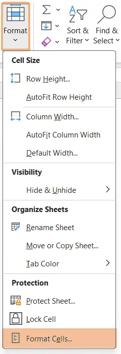
1. Go to the Format tool under the Cells group.
2. Then, select Format Cells command.
   
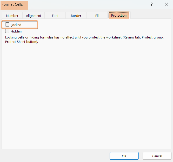
3. Next, navigate to the Protection tab in the Format Cells dialog box.
4. Now, uncheck the Locked option and click OK.
   

Step 2: Protect Your Excel Sheet

As we disabled the Locked options, now we need to Protect Worksheet. To do that, follow the steps below:

1. Navigate to Review tab > Protect Sheet under Protect group.
   
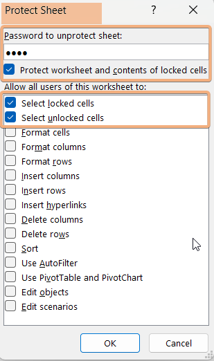
2. Then, insert the password to unprotect the sheet.
3. Next, check on the Select locked cells and Select unlocked cells and click OK.
   

This will lock the Pivot Table layout. You can’t make any changes to the Pivot Table until you unprotect the Pivot Table.

Using VBA Code to Lock Pivot Table Column Width in Excel

You can lock the Pivot Table column width by applying the VBA code in Excel. Follow the steps to run the VBA code:

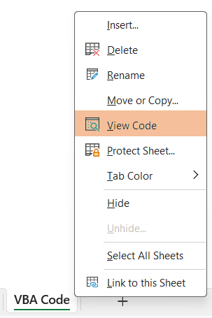
1. Go to the sheet’s name and select View Code.
   
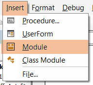
2. Then, go to Insert tab > Module option.
   
3. Copy and Paste the VBA Code below:

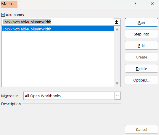
   Sub LockPivotTableColumnWidthWithUserInput()
   
       Dim ws As Worksheet
       Dim pivotTable As pivotTable
       Dim targetRange As Range
       Dim userPassword As String
       Dim columnWidth As Double
       ' Set the worksheet
   
       Set ws = ThisWorkbook.Sheets("VBA Code") ' Replace "VBA Code" with the actual sheet name
   
       ' Set the target range (columns in the pivot table)
       Set targetRange = ws.PivotTables("PivotTable1").TableRange1 ' Replace "PivotTable1" with the actual pivot table name
   
       ' Prompt the user for a password
       userPassword = InputBox("Enter the password to protect the worksheet", "Password")  
   
       ' Exit if the user clicks Cancel
   
       If userPassword = "" Then
   
           Exit Sub
       End If
       ' Prompt the user for the column width
   
       columnWidth = InputBox("Enter the desired column width", "Column Width")
       ' Exit if the user clicks Cancel or enters an invalid width
   
       If columnWidth <= 0 Then
           Exit Sub
       End If   
   
       ' Unlock all cells on the worksheet
       ws.Cells.Locked = False
   
       ' Set the column width for the target range
       targetRange.columnWidth = columnWidth
   
       ' Lock the cells in the target range
       targetRange.Locked = True
       ' Protect the worksheet with the user-entered password
       ws.Protect Password:=userPassword, UserInterfaceOnly:=True
   
   End Sub

4. Now, press ALT+F8 to open the Macro dialog box and click Run.
   
   
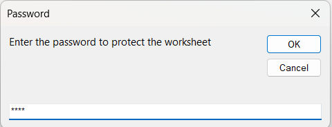
5. After clicking on Run, insert a password to protect the sheet and click OK.
   
6. Now, enter the column width and click OK.
   After clicking OK, you will see the updated column width as your input in Excel. Besides that, it will lock the Excel worksheet until you unprotect it.

Shortcut Keys to Autofit Column Width in Excel

After turning off the “Autofit Column Width on update”, you may need to turn on that option again. Now, you can turn it on by navigating to Home tab > Format tool > Autofit Column Width. Or, use the shortcut key ALT+H+O+I to autofit the column width in Excel.

Conclusion

When you make any changes in the Pivot Table, it updates the column width in the Pivot Table. However, it will be hectic while working on shapes, charts, and slicers outside the Pivot Table. So, you have to lock the Pivot Table column width in Excel. In this article, I have added 3 ways to lock the Pivot Table column width in Excel. Additionally, I have also added a shortcut to enable Autofit Column Width in Excel. Hopefully, you won’t face any problems regarding locking the Pivot Table column width after going through this article.

Frequently Asked Questions

How do I maintain a pivot table format?

To maintain a PivotTable format in Excel, follow these steps:

1. Preserve Cell Formatting: Before creating the Pivot Table, ensure that the Preserve cell formatting on update option is enabled. You can find this option by right-clicking on the PivotTable, selecting PivotTable Options, and checking the box for Preserve cell formatting on update.
2. Apply Conditional Formatting to Source Data: If you’re using conditional formatting in your Pivot Table, apply the same formatting to the source data. This ensures that when the PivotTable is refreshed, the formatting remains consistent.
3. Use PivotTable Styles: Utilize built-in PivotTable Styles in Excel. These styles not only enhance the visual appeal of the Pivot Table but also help maintain a consistent format. You can find and apply styles in the Design tab when the Pivot Table is selected.

By following these steps, you can help ensure that the formatting of your Pivot Table is preserved even after refreshing or updating the data.

How do I format a pivot column?

To format a column in a Pivot Table in Excel, follow these steps:

1. Click on any cell within the column you want to format in the Pivot Table.
2. Navigate to the Home tab on the Ribbon at the top of the Excel window.
3. Use the formatting options available in the Number groups to format the selected column. Common formatting options include Number, Font, and Alignment.
4. Apply conditional formatting to highlight specific data trends or values within the column. You can do this through the Conditional Formatting option in the Home tab.
5. If you want to maintain formatting consistency, consider formatting the source data itself. Any formatting applied to the source data will carry over to the Pivot Table.
6. Explore the Design tab in the Ribbon, where you can find predefined PivotTable styles. Applying a style can enhance the overall appearance of the Pivot Table, including formatted columns.

By following these steps, you can easily format a column within a Pivot Table to meet your specific visual and analytical requirements in Excel.

How do you freeze a pivot table layout?

To freeze a Pivot Table layout in Excel and keep specific rows or columns visible while scrolling, follow these steps:

1. Click on any cell within the PivotTable that corresponds to the row or column you want to freeze.
2. Navigate to the View tab on the Ribbon at the top of the Excel window.
3. In the Window group on the View tab, click on the Freeze Panes dropdown. Then, select the Freeze Panes option from the dropdown menu.

This will freeze the rows above and columns to the left of the selected cell. If you want to freeze specific rows or columns, select the cell in the row below the rows you want to freeze or the column to the right of the columns you want to freeze. To unfreeze panes, go back to the Freeze Panes dropdown and select Unfreeze Panes.

How do you preserve row height in a pivot table?

Preserving row height in a Pivot Table can be crucial for maintaining a consistent and organized appearance. Follow these steps in Excel to preserve row height:

1. Click on the triangle between the row and column headers (top-left corner) to select the entire worksheet.
2. Adjust row heights by right-clicking on any selected row number, and choosing Row Height from the context menu.
3. Enter the desired row height in the Row Height dialog box.
4. Ensure that the Preserve cell formatting on update option is enabled. Right-click on the PivotTable, go to the PivotTable Options, and check this option under the Layout & Format tab.

By following these steps, you can set and preserve row heights in a Pivot Table, ensuring a consistent and visually appealing layout, even when refreshing or updating the data.