How to Find Second Match in Excel Using XLOOKUP [4 Methods]
Follow these steps to find the second match in Excel using XLOOKUP:
- Choose cell E3.
- Type the formula: =XLOOKUP(E1&E2, A2:A10&SORTBY(SEQUENCE(ROWS(A2:A10),1,2)-MATCH(SORT(A2:A10),SORT(A2:A10),0),SORTBY(SEQUENCE(ROWS(A2:A10),1,2),A2:A10,1),1),B2:B10)
- Hit ENTER to see the result.
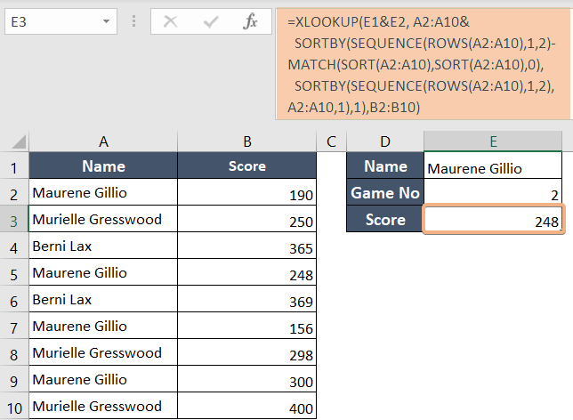
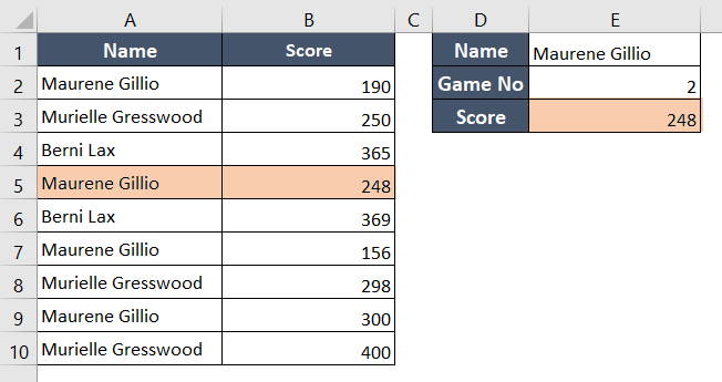
This formula looks for the second occurrence of “Maurene Gillio” by combining the contents of cells E1 and E2 in a list (A2:A10). To make this search efficient, it sorts the list in a special way. When it finds the position of the combined value in the sorted list, it retrieves the matching value “248” from the range B2:B10 using the XLOOKUP function.
1. Find the Second Match Using the XLOOKUP Function in Excel
XLOOKUP is a powerful function in Microsoft Excel that allows you to search for a specific value in a column and retrieve a corresponding value from another column.
In this case, I want to find the second match of the “Maurene Gillio” from the “Name” column and retrieve the corresponding 2nd match value from the “Score” column.
Syntax
=XLOOKUP(lookup_value&nth, lookup_array&nth_lookup_array, return_array)Formula
=XLOOKUP(E1&E2, A2:A10& SORTBY(SEQUENCE(ROWS(A2:A10),1,2)-MATCH(SORT(A2:A10),SORT(A2:A10),0), SORTBY(SEQUENCE(ROWS(A2:A10),1,2),A2:A10,1),1),B2:B10)Formula Breakdown
- This Excel formula employs the XLOOKUP function to search for a value created by concatenating the contents of cells E1 and E2 within a specific range (A2:A10).
- The formula uses advanced sorting techniques, including custom sorting orders generated by the SORTBY and SEQUENCE functions, to optimize the lookup process.
- The MATCH function is utilized to identify the position of the search value within a sorted array (A2:A10 after sorting). It determines the relative position of the concatenated value in the sorted list.
- Once the match position is found, XLOOKUP retrieves the corresponding value from the range B2:B10, providing a powerful way to perform a customized, sorted lookup based on the concatenated values of E1 and E2.
Use the XLOOKUP function to find the second match in Excel. Follow the steps below:
- Select cell E3.
- Copy this formula: =XLOOKUP(E1&E2, A2:A10& SORTBY(SEQUENCE(ROWS(A2:A10),1,2)-MATCH(SORT(A2:A10),SORT(A2:A10),0), SORTBY(SEQUENCE(ROWS(A2:A10),1,2),A2:A10,1),1),B2:B10)
- Press ENTER.

Final Result
The second occurrence of “Maurene Gillio” has been located, and it corresponds to the value “248.”
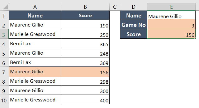
You can also use this function to find the “n-th” match. For example, if you need to locate the third occurrence, simply input “3” into cell “E2,” and the function will automatically identify the third match.
2. Lookup Vertically to Get the Second Match Using FILTER Function in Excel
The FILTER function in Excel is a useful tool for extracting data according to predetermined standards. For different data analysis jobs, finding the second match using FILTER helps identify the second instance of a condition inside a dataset.
Syntax
=INDEX(FILTER(array,include),row_number)Formula
=INDEX(FILTER(B2:B10,A2:A10=E1),E2)Formula Breakdown
- This Excel formula first filters the values in column B (B2 to B10) based on a condition in column A (A2 to A10) where it matches the value in cell E1. The FILTER function extracts values from B2:B10 that correspond to the condition specified in A2:A10.
- It then uses the INDEX function to retrieve the value at the location indicated in cell E2 from the filtered list. Essentially, it fetches the value in the filtered list corresponding to the row specified by E2.
Utilize the FILTER function to vertically lookup the second match in Excel. The process is outlined below:
- Select cell E3.
- Use this formula: =INDEX(FILTER(B2:B10,A2:A10=E1),E2)
- Press ENTER to see the result.

Final Result
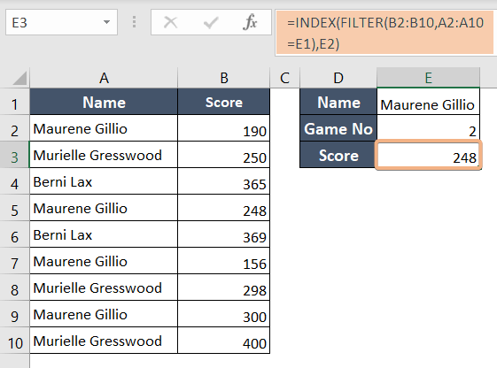
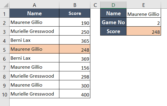
This formula combines INDEX and FILTER functions to extract specific values, like ‘Maurene Gillio,’ and find their second occurrence in a list.
3. Locate the Second Match in Excel Using the INDEX and AGGREGATE Function
When working with a dataset in Excel, the INDEX and AGGREGATE functions can be used to quickly locate and obtain the second instance of a certain value or condition.
Syntax
=INDEX(array,AGGREGATE(function_number,options,(ROW(ref_1)/(ref_2),[k]))Formula
=INDEX(B2:B10,AGGREGATE(15,6,(ROW(A2:A10)-1/(A2:A10=E1),E2))Formula Breakdown
- This formula combines the INDEX and AGGREGATE functions to perform a data lookup in Excel. It extracts data from the range B2:B10. The AGGREGATE function works by identifying the row number of a specific value in column A (A2:A10) that matches the value in cell E1.
- It does this by calculating the position based on the ROW function, adjusted for matches with the expression (1/(A2:A10=E1)). The ROW function generates an array of row numbers for the range A2:A10, and the expression (1/(A2:A10=E1)) produces an array of 1s and errors, with 1s in positions where A2:A10 matches the value in cell E1.
- The AGGREGATE function then uses its arguments (15 and 6) to ignore errors, sort the resulting array, and return the ‘k-th’ smallest value, which, in this case, is the row number where the first match occurs.
- The result from AGGREGATE, which represents the row number, is then used with INDEX to retrieve the corresponding value from the range B2:B10. Essentially, it fetches the data from B2:B10 that corresponds to the row number of the first occurrence of the value in cell E1 in the range A2:A10.
Use a combination of INDEX and AGGREGATE functions to vertically look up the second match in Excel. Here’s how:
- Choose cell E3.
- Write the formula: =INDEX(B2:B10,AGGREGATE(15,6,(ROW(A2:A10)-1/(A2:A10=E1),E2))
- Press ENTER.

Final Result
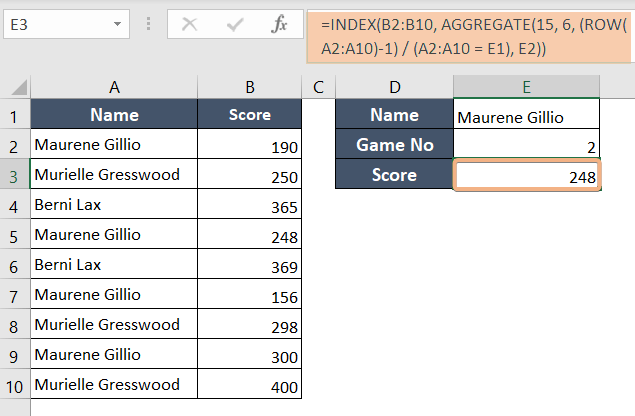
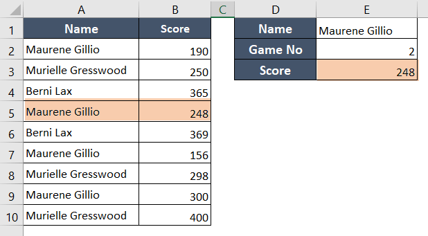
The INDEX and AGGREGATE functions work together to locate and extract the value “248” associated with the second instance of the condition “Maurene Gillio”.
4. Using IF and SMALL Functions to Lookup the Second Match in Excel
Here, I have employed the IF and SMALL functions to locate the second match efficiently.
Syntax
=INDEX(array, SMALL(IF(logical_test, reference, k))Formula
=INDEX(B2:B10, SMALL(IF(A2:A10=E1, ROW(A2:A10)-ROW(A2)+1), E2))Formula Breakdown
- This formula combines the INDEX and SMALL functions to extract a value from the range B2:B10. It begins by using the IF function to check if values in the range A2:A10 match the content of cell E1 and, if they do, it generates an array of corresponding row numbers.
- The ROW function assists in creating this array of row numbers. Subsequently, the SMALL function retrieves the value from cell E2, which represents the position of the desired value within the B2:B10 range. Finally, the INDEX function employs this row number to fetch the corresponding value.
Utilize a combination of IF and SMALL functions to vertically look up the second match in Excel. Follow the steps below:
- Select cell E3.
- Type the formula: =INDEX(B2:B10, SMALL(IF(A2:A10=E1, ROW(A2:A10)-ROW(A2)+1), E2))
- To insert the formula press ENTER.

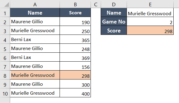
Final Result
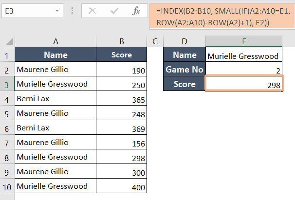
After applying this formula, we find the expected result.
Conclusion
In this article, I’ve discussed four methods to discover the second match in Excel. Typically, the XLOOKUP function is employed to search for a value within a range and retrieve a corresponding value from another range. Moreover, XLOOKUP can also be utilized to find the “n-th” match in Excel.
Frequently Asked Questions
How do I find my second instance in XLOOKUP?
To find the second instance in XLOOKUP in Excel, use the SMALL function within an array formula. Here’s a sample formula:
=XLOOKUP(lookup_value, lookup_array, return_array, , , SMALL(IF(lookup_array=lookup_value, ROW(lookup_array)-MIN(ROW(lookup_array))+1), 2))- Press Ctrl+Shift+Enter to apply the formula.
- Adjust ‘lookup_value’, ‘lookup_array’, and ‘return_array’ as needed.
What if XLOOKUP has multiple matches?
If XLOOKUP in Excel has multiple matches, it returns the first match it encounters. For all matches, consider using INDEX and MATCH or array formulas.
Can you do a double XLOOKUP?
Excel’s XLOOKUP doesn’t support a direct ‘double XLOOKUP.’ To achieve a similar result, you can use other methods like INDEX and MATCH.
- Use the formula: =INDEX(return_array, MATCH(lookup_value1 & lookup_value2, criteria_array1 & criteria_array2, 0))
- Concatenate the criteria (lookup_value1 and lookup_value2).
- Compare the concatenated criteria with the concatenated criteria in the data (criteria_array1 and criteria_array2).
- MATCH finds the position of the match.
- INDEX retrieves the corresponding result from return_array.
How do I select a second value in VLOOKUP?
In a standard VLOOKUP function in Excel, you cannot directly select a second value. VLOOKUP is designed to return the first match it finds based on a specified lookup value. If you need to retrieve a second value, you may consider using alternative methods.
If you want to select a second value in Excel, consider using the INDEX and MATCH functions for a more versatile lookup process. Example: =INDEX(B:B, MATCH(D1, A:A, 0) + 1)
