How to Edit Pivot Table Calculated Field [Step-by-Step]

To edit Pivot Table Calculated Fields, go through the steps below:

1. Click any cell in the Pivot Table to access PivotTable Tools.
2. Navigate to the Analyze tab.
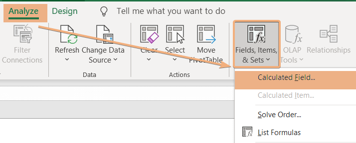
3. Access the Fields, Items & Sets dropdown > Calculated Field option.
4. Select the existing calculated field in the Insert Calculated Field dialog box.
5. Modify the formula in the Formula box with the desired changes.
6. Click Modify and then OK.

By following the above-mentioned process, edit the Pivot Table Calculated Field and enhance your data analysis capabilities.

Step 1: Prepare Dataset and Insert Pivot Table in Excel

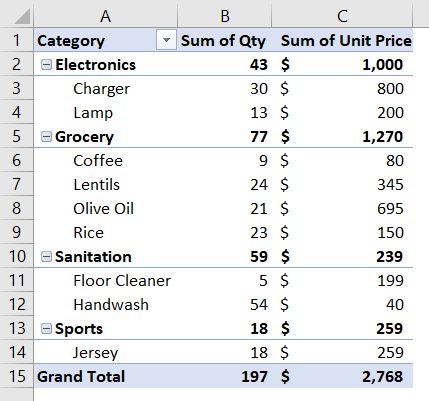
In this approach, I have a dataset of the unit price of some products. Additionally, we have a list of categories and quantities for each product. Now, I will create a sales report in a Pivot Table.

To insert a Pivot Table in Excel, follow the steps below:

1. Select the entire range.
2. Go to Insert tab > PivotTable dropdown > From Table/Range option.
   
3. Confirm the range and choose the location to place the Pivot Table.
4. Click OK.
   

Now, you have inserted a Pivot Table in Excel. Then, we will organize the Pivot Table.

Step 2: Create a Pivot Table and Arrange with PivotTable Fields

In this part, we will create the Pivot Table by organizing the Pivot Table with PivotTable Fields in Excel.

1. Click on a cell in the Pivot Table.
2. Go to the PivotTable Fields.
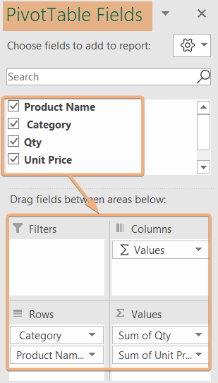
3. Choose fields from the list.
4. Then, drag and put it into the areas, Rows, Columns, Filters, and Values.
   Here, I have added the category with the product name in the Rows area. Then, I put the quantity and unit price in the Values area.
   

So, I have created the Pivot Table eventually.

Step 3: Insert a Formula in the Pivot Table Calculated Field

In this step, I will insert a formula in the Pivot Table Calculated Field in Excel. Here is the procedure below:

1. Select any cell within the Pivot Table.
2. Go to the PivotTable Tools > Analyze tab.
3. Now, click the dropdown of Fields, Items & Sets > Calculate Field option.
   
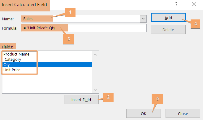
4. In the Insert Calculated Field dialog box, enter a name.
5. Choose fields from the list and click Insert Field option.
6. Insert the formula in the Formula box.
7. Click on Add and hit OK.
   

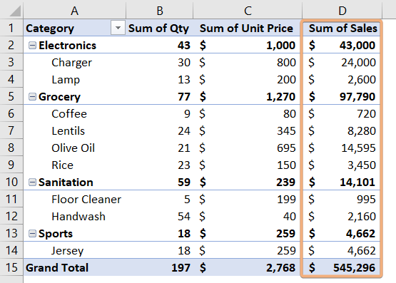
You can see the inserted calculated field in the Excel Pivot Table. Here is an added column with the entered formula in the Pivot Table Calculated Field.

Step 4: Edit Pivot Table Calculated Field

If you insert a formula wrong in the inserted calculated field, then you can also modify the Pivot Table Calculated Field. Now, I want to edit the formula. Here’s how:

1. Click on any cell in the Pivot Table.
2. Navigate to the Analyze tab in the PivotTable Tools.
3. Go to Fields, Items & Sets dropdown > Calculated Field option.
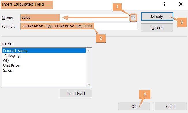
4. Select the name of the inserted calculated field in the Insert Calculated Field dialog box.
5. Then, insert the new formula in the Formula box with the fields list.
6. Click on Modify.
7. Hit OK.
   

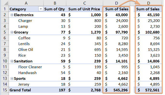
By doing these steps, you will able to edit the Calculated Field in the Excel Pivot Table. Now, notice the change in the Excel Pivot Table in the image.

Conclusion

In conclusion, editing a calculated field in a Pivot Table is a straightforward process that allows users to refine and customize their data analysis. So, in this article, I have added a step-by-step approach to editing a Pivot Table Calculated Field. You will learn to insert a Pivot Table from a data range first. Then, you will able to create a Pivot Table by choosing fields, and next adding a formula in the calculated field. So, go through this article and explore to edit the Pivot Table in the Calculated Field.

Frequently Asked Questions

Why do we use a calculated field?

A calculated field in a Pivot Table is used to perform calculations on existing fields and create new ones based on specific formulas. It helps users derive meaningful insights and analyze data more efficiently. Calculated fields are valuable for summarizing, comparing, or transforming data within the Pivot Table, providing a dynamic way to explore and interpret information. They are especially useful when standard aggregation functions do not meet specific analytical requirements, allowing users to customize their data analysis.

Why can’t I add a calculated field to PivotTable?

If you can’t add a calculated field to a PivotTable, check the following:

• Data Format: Ensure your data is in a tabular format with column headers. Calculated fields require well-structured data.
• Blank Cells: Remove any blank cells in the data as they might hinder the calculation process.
• Unique Field Names: Make sure there are no duplicate field names, as this can cause conflicts.
• Valid Formulas: Double-check the syntax and validity of your calculated field formula.
• PivotTable Structure: Confirm that the PivotTable layout allows the addition of calculated fields.

By addressing these issues, you should be able to add a calculated field successfully.

How do I show different calculations in a Pivot Table value field?

To show different calculations in a Pivot Table value field, follow these steps:

1. Click on any cell within the Pivot Table.
2. Navigate to the PivotTable Analyze tab.
3. In the Value Field Settings dialog box, select the field.
4. Choose the summary function you want.
5. Duplicate the value field and choose different summary functions.
6. Click OK to apply the changes.
7. Refresh the Pivot Table.

By following these steps, you can show various calculations in a Pivot Table value field.