3 Methods to Convert Column Number to Letter in Excel

Usually, if you open an Excel workbook, the column headers are supposed to stay alphabetically. If the columns are in numbers in your worksheet, here are 3 methods to convert a column number to a column letter in Microsoft Excel.

Here’s the Excel file that I’ve used throughout the whole blog. You can download it from the following link:

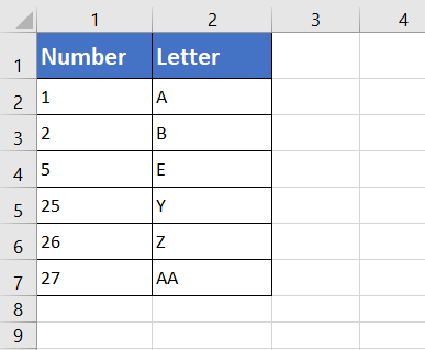
Before moving to the solutions, let me introduce you to the dataset I used for this blog. I have used a simple dataset where I’ve put some numbers (column: Number) by the serial of the alphabet (column: Letter).

Convert Excel Column Number to Letter Using Built-in Option

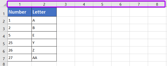
You can see the column headers are in numbers. Now, I am going to use the built-in option of Microsoft Excel to change the column header numbers to column letters.

To convert Excel column number to letter with built-in option, follow these steps below:

1. Click on the File menu.
2. Select Options.
   
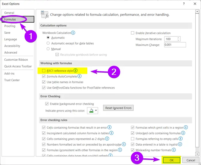
   The Excel Options dialog box will pop up.
3. Select Formulas.
4. From the Working with Formulas group, unmark the R1C1 Reference Style checkbox.
5. Hit OK.

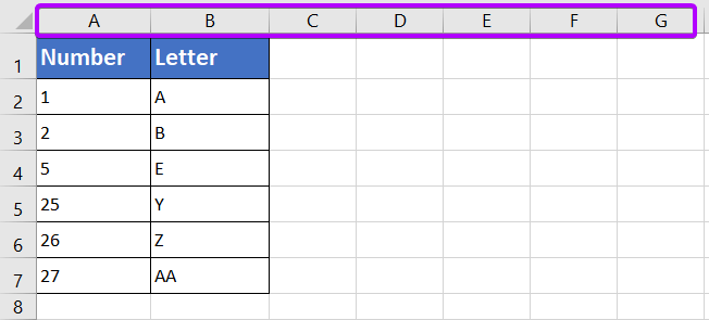
Now, you will find the column headers in ABCD forms.

Note:

Let’s say, you had another workbook open while working with your current workbook, you would see the other workbook had also switched its reference style into lettered column headers.

To avoid this problem, I would suggest, opening the workbooks one by one. Or, you can again change the settings in the Options into the R1C1 reference style.

• 3 Ways to Find Column Index Number in Excel
• 2 Ways to Count Columns in Excel for Vlookup

Convert Column Number to Letter to Use ADDRESS Function in Excel

This formula is applicable for any column number. It has no limitation on column counting. So, it’s very useful.

Formula Syntax

=ADDRESS(row_number, column_number, [absolute_num], [a1], [sheet text])

Formula

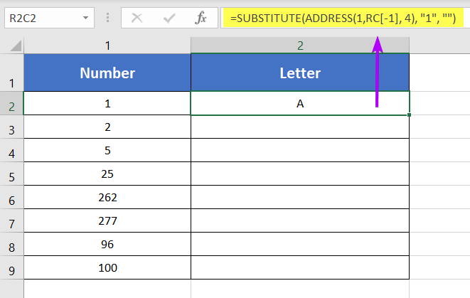
=SUBSTITUTE(ADDRESS(1,RC[-1], 4), "1", "")

Formula Explanation

The ADDRESS function requires a row number and a column number as input. It merges the input values and returns a cell address as an output. Inside the ADDRESS function,

• 1 is the row number. Then RC[-1] is the column number.
• RC[-1]: Here, R refers to the same row as the active cell which is row 1. Then, C[-1] refers to the immediate left column of the active cell which is column 1.
• 4 is the serial number of Relative Cell Reference.

Thus, ADDRESS(1,RC[-1], 4) returns A1.

Then, the SUBSTITUTE function requires a text. Where it replaces an old text with a new text.

• The ADDRESS function returns A1. This A1 is the input text for the SUBSTITUTE function.
• “1” is the old text here.
• “” is the new text.

Thus, the SUBSTITUTE function replaces 1 with a null string and A1 becomes A.

Apply ADDRESS function to convert column number to letter. So, go through these following steps:

1. Select a blank cell.
2. Type this formula: =SUBSTITUTE(ADDRESS(1,RC[-1], 4), “1”, “”)
   
   
3. Press ENTER.
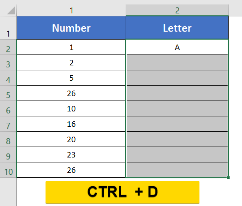
4. Select the whole column.
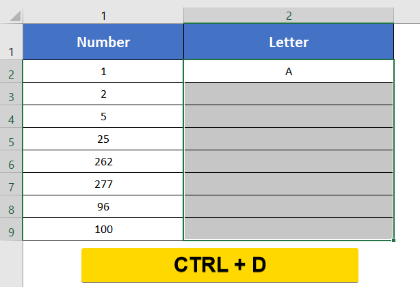
5. Press CTRL + D.
   This will copy down the formula applied in the top cell of the column, Letter.

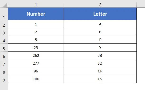
Input numbers are converted into column letters. Take a look.

• [2 Cases] Count Columns in Excel Until a Certain Value Reached
• Count Rows in Excel Until a Certain Value Reached [2 Cases]

Convert Column Number to Letter Using CHAR Function

Before moving into this method, let me notify you that this technique is only applicable if you are looking for a column number that is within range of the 26 alphabets. Not applicable for header numbers above 26.

Formula Syntax

=CHAR(64 + column_number)

Formula

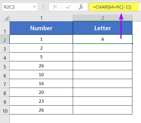
=CHAR(64+RC[-1])

Formula Explanation

CHAR function requires a number. Then, it converts the number to its corresponding character. R refers to the same row as the active cell which is 1. C[-1] refers to the immediate left column of the active cell’s column; which is column 1. Thus, RC[-1] refers to the first cell of the column, Number; which contains the number 1. CHAR function receives numbers from 1 to 26. When 64 is added to the range (1 to 26), we get a range of 65 to 90. 65 is the ASCII equivalent number of the letter ‘A’. 90 is the ASCII equivalent number of the letter ‘Z’.  Thus, the CHAR function converts 1 to 26 as ‘A’ to ‘Z’.

Go through the steps to convert column number to letter using CHAR function:

1. Select an empty cell.
2. Type this formula: =CHAR(64+RC[-1])
3. Press ENTER key.
   
   
4. Select the entire column.
5. Now, press CTRL + D.
   This will instantly copy down the formula applied in the top cell with changing cell reference.

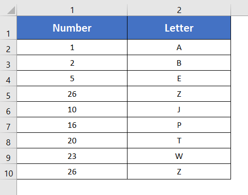
All the numbers from 1 to 26 have been converted into column letters. Have a look:

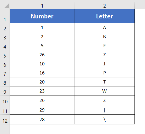
In case you try a column number above 26, Excel will give you a result based on the ASCII coding system.

• 6 Ways to Count One Column in Excel If Another Column Meets Criteria
• [Excel VBA] Count Columns & Rows Having Data (10 Editable Codes)

Conclusion

I hope now you have a clear idea about converting column headers numbers and column letters, and can solve any problems regarding this topic. Please feel free to reach out to us, if you have any confusion regarding this article.

Frequently Asked Questions

How do I turn on R1C1?

To turn on R1C1 reference style in Excel, follow these steps:

1. Click on the File tab in the Excel ribbon.
2. Select Options at the bottom of the menu to open the Excel Options dialog box.
3. In the Excel Options dialog box, click on the Formulas category in the left sidebar.
4. Look for the Working with formulas section and find the R1C1 reference style option.
5. Check the box next to R1C1 reference style to enable it.
6. Click OK to apply the changes.

By following these steps, you can easily switch to R1C1 reference style in Excel, which represents cells by their row and column numbers, providing an alternative to the default A1 reference style.

How do I get rid of R1C1 in Excel?

To disable R1C1 reference style in Excel, follow these simple steps:

1. Click on the File tab in the Excel ribbon.
2. Select Options at the bottom of the menu to open the Excel Options dialog box.
3. In the Excel Options dialog box, click on the Formulas category in the left sidebar.
4. Locate the Working with formulas section and uncheck the box next to R1C1 reference style.
5. Click OK to apply the changes.

By following these steps, you can easily revert to the default A1 reference style in Excel and eliminate the use of R1C1. This restores the conventional cell addressing format for a more familiar and user-friendly experience.

How do you convert a column letter to a column number in Excel?

To convert a column letter to a column number in Excel, use the following formula:
=COLUMN(A:A) – COLUMN(A$1) + 1
Replace ‘A’ with the target column letter. This formula subtracts the column number of the first column from the column number of the target column, then adds 1. The result is the corresponding column number. This approach is particularly useful for dynamic column referencing in Excel formulas, allowing seamless conversion between letters and numbers for improved flexibility in spreadsheet calculations.