How to Change Pivot Table Layout in Excel [5 Best Methods]
5 Methods to Change Pivot Table Layout in Excel
Initially, I have created a Pivot Table with default settings. Next, I want to change the Pivot Table Layout in Excel.
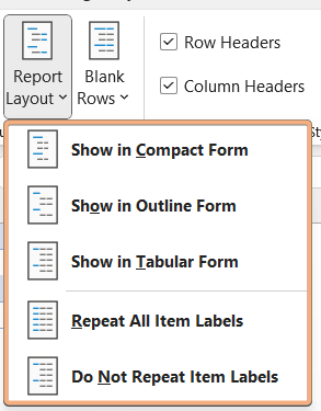
To change the Pivot Table layout in Excel, go through the process below:
- Click on any cell in the Pivot Table.
- Navigate to the Design tab.
- Then, hit the dropdown Report Layout.
- Now, choose the layout form from the list of Report Layout.

Using Report Layout Options to Display Pivot Table Form in Excel
If you create a pivot table, you can access the Design tab by clicking on any cell in the Pivot Table. Then, you will see the Report Layout option to change the Pivot Table layout. Now, we will see how the Pivot Table view changes with each type of layout.
Case 1: Show in Compact Form
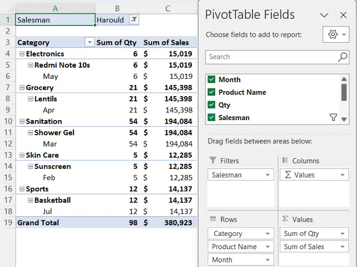
From the Report Layout option, choose Show in Compact Form option. Usually, it is the default form of a Pivot Table. You will see all the row labels in a single column.
In the image, you can see the Pivot Table shown in compact form in Excel.
Case 2: Show in Outline Form
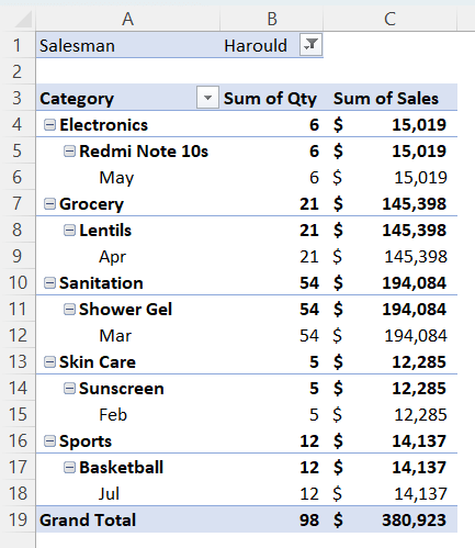
To access this option, go to the Design tab clicking on Pivot Table. Then, select Show in Outline Form option. Here, each row label will be in a separate column.
Finally, you will see the changing layout of your pivot table in Excel. However, the following columns of the first column will be as subsections in outline form in the Pivot Table.
Case 3: Show in Tabular Form
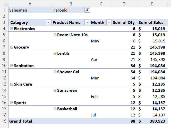
To make your Pivot Table more organized, you can change the Pivot Table layout to Show in Tabular Form from the dropdown list of Report Layout in Excel.

Using Report Layout Options to Display All Item Labels in Excel
In Report Layout options, you can choose to repeat all item labels in each column or not to repeat any in Excel.
Case 1: Repeat All Item Labels
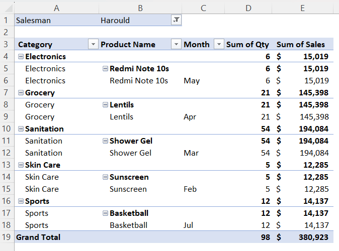
See the Pivot Table with repeating all item labels in Excel. To see that view, go to Design tab > Report Layout tool > Repeat All Item Labels option.
In the image, you can see repeated item labels in Excel in each row of that item.
Case 2: Do Not Repeat Item Labels
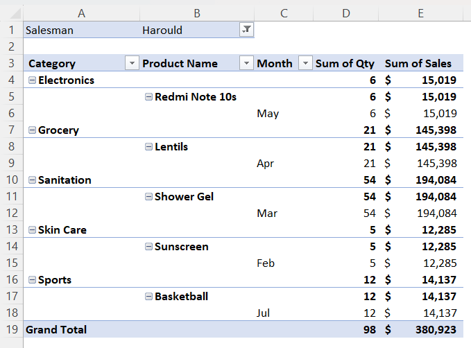
You can also choose not to repeat item labels in Excel. To visualize that, choose Do Not Repeat Item Labels from Report Layout tool in the Design tab in Excel.
By doing these, Excel will not show the item labels in each row in the Pivot Table.
Using Blank Rows Option to Change Pivot Table Layout in Excel
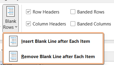
The Blank Rows option in Pivot Table usually inserts or removes a blank row after each item details to change the Pivot Table layout in Excel.
Case 1: Insert a Blank Line after Each Item
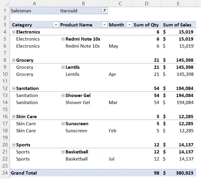
If you choose Insert Blank Line after Each Item from Blank Rows dropdown, Excel will update the Pivot Table.
Case 2: Remove the Blank Line after Each Item
To remove these inserted blank rows after each item, click on the Remove Blank Line after Each Item in Excel.
Using Subtotals Options to Change Pivot Table Layout in Excel
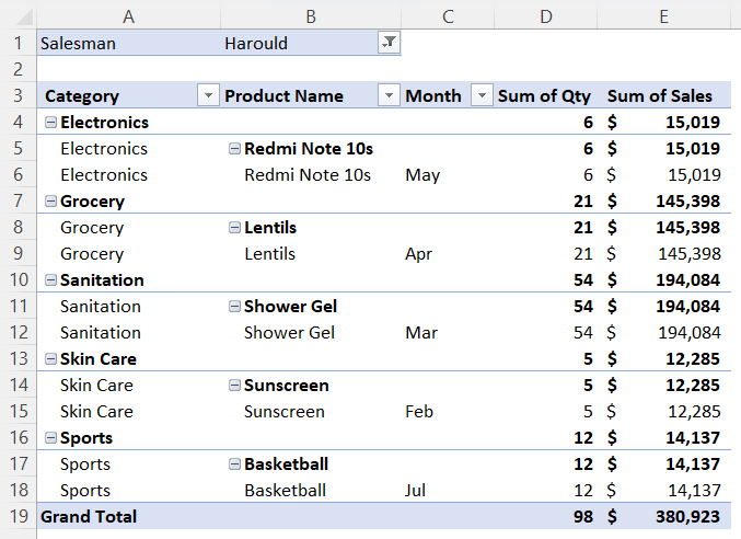
After accessing the Design tab in Excel, you will see the Subtotals tool to show the subtotal values top or bottom of the group or not showing subtotals at all.
Case 1: Do Not Show Subtotals
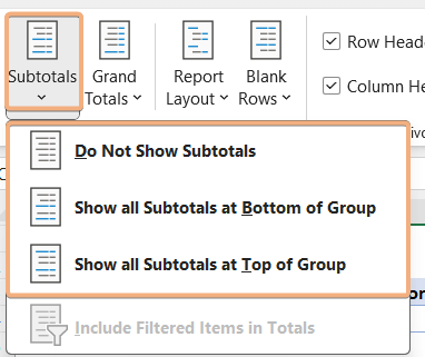
To change the Pivot Table layout using this option, click anywhere in the Pivot Table first. Then, access the Design tab and hit the dropdown of Subtotals. Next, choose Do Not Show Subtotals option.
In this image, you will see the changed Pivot Table layout in Excel. Here, it does not show any subtotals in each row. Rather it shows the total value in a row of each item.
Case 2: Show all Subtotals at Bottom of Group
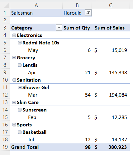
To access this option, go to the Design tab. Then, choose Show all Subtotals at Bottom of Group option under the Subtotals option. It shows subtotals at the bottom of each item group.
Case 3: Show all Subtotals at Top of Group
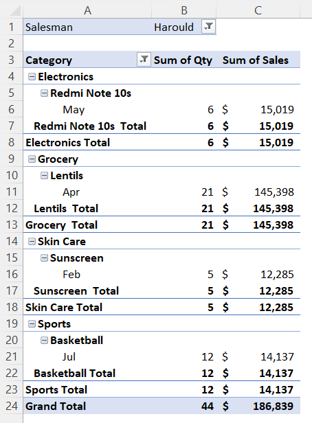
Usually, according to the default settings, you will see the subtotals at the top of each item group. If you want to change the Pivot Table layout to this, click on the Pivot Table to navigate to the Design tab. Then, select Show all Subtotals at Top of Group option under the Subtotals tool.
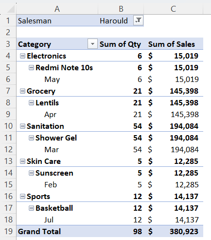
Using Grand Totals Options to Change Pivot Table Layout in Excel
In a Pivot Table, there is a Grand Totals value at the end of each numerical column, such as the sum of sales, the sum of quantity, etc. You can change the Pivot Table layout by choosing these 4 options to show or hide grand totals in the Pivot Table.
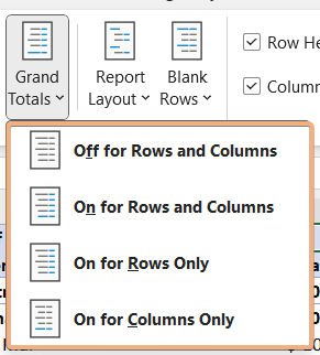
Case 1: Off for Rows and Columns
To choose this option, go to the Design tab by clicking on a cell in the Pivot Table. Now, select Off for Rows and Columns option. It will change the Pivot Table layout by turning off the grand totals from both rows and columns.
You can see the screenshot, there is no Grand Total column or row in the Pivot Table.
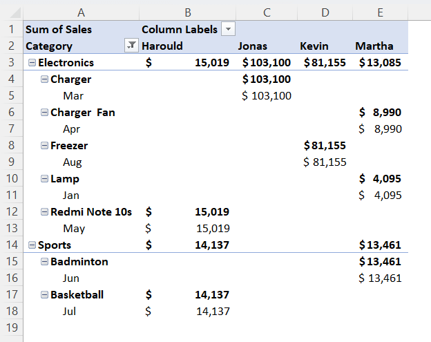
Case 2: On for Rows and Columns
Choose On for Rows and Columns from Grand Totals in the Design tab. After enabling this option, it will add a column of Grand Total at the right and a row of Grand Total at the bottom.
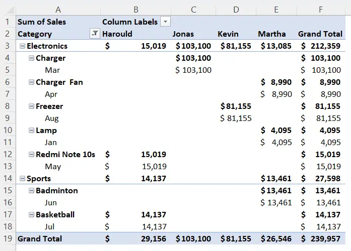
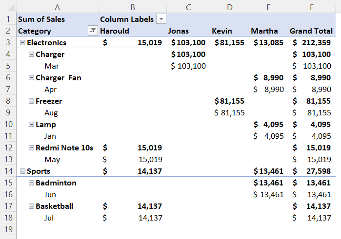
Case 3: On for Rows Only
Navigate to the Design tab > Grand Totals tool > On for Row Only option. It will enable the Grand Total only for the rows. Hence, it will add a column at the right in the Pivot Table.
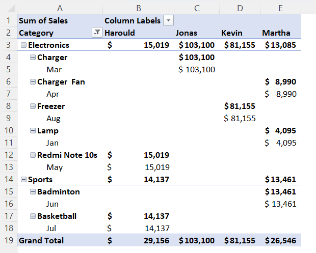
Case 4: On for Columns Only
Now, to enable the Grand Total only for the columns, Design tab > Grand Totals tool > On for Row Only option. Therefore, it will add a row at the bottom of the Pivot Table.
Conclusion
Pivot Table is a flexible tool for data summarization and analysis in Excel. Excel also offers to change the Pivot Table layout to visualize the data more concisely. So, in this article, I have added the step-by-step guide to change the Pivot Table layout in Excel. Then, I have also described the options to choose from Report Layout, Blank Rows, Subtotals, Grand Totals to change the Pivot Table layout. Hopefully, you will get a detailed guideline to change the Pivot Table layout in Excel.
Frequently Asked Questions
What is Pivot Table layout?
The Pivot Table layout in Excel refers to the arrangement and organization of fields and data within a Pivot Table. It determines how the data is presented for analysis and reporting. The layout typically consists of the following areas:
- Rows: Fields placed in the Rows area are used to categorize and group data along the vertical axis. This is where you define the primary criteria for your analysis.
- Columns: Fields placed in the Columns area are used to categorize and group data along the horizontal axis. They allow you to create side-by-side comparisons.
- Values: Fields placed in the Values area contain the data that you want to summarize, such as sums, averages, or counts. These fields provide the actual metrics of your analysis.
- Filters: Fields placed in the Filters area allow you to filter and limit the data displayed in the Pivot Table based on specific criteria or conditions.
By arranging fields in these areas, you can control the layout of your Pivot Table to best suit your data analysis needs, making it easier to interpret and present information effectively.
How do I change a Pivot Table to the classic view?
To change a Pivot Table to the Classic View Layout, go through the instructions below:
- Click any cell in the Pivot Table.
- Go to PivotTable Analyze tab > Options under the PivotTable group.
- Then, navigate to the Display tab in the PivotTable Options dialog box.
- Next, check on Classic PivotTable Layout.
- Click OK to apply the classic layout to your Pivot Table.
Following these steps will configure your Pivot Table to use the Classic PivotTable Layout, which may resemble older versions of Excel or provide a more traditional appearance.
How do I change the default view in a Pivot Table?
To change the default view in a Pivot Table in Excel, you can follow these steps:
- Click anywhere within the Pivot Table to select it.
- Go to the PivotTable Analyze tab on the Excel ribbon.
- In the PivotTable Options section, you can customize various settings to change the default view. These settings include:
Gridlines: You can toggle gridlines on or off to change the appearance of the Pivot Table.
Subtotals: You can choose how subtotals are displayed in the Pivot Table.
Report Layout: You can select different layout options, such as tabular, outline, or compact, to change the default view. - Adjust the settings according to your preferences.
By changing these settings, you can modify the default view of your Pivot Table to match your desired appearance and layout.
