How to Connect Two Slicers in Excel [Step-by-Step]

A slicer is a visual control element that facilitates the filtering of data in a Pivot Table or Pivot Chart. Slicers provide an intuitive and user-friendly way to interact with large datasets, allowing users to dynamically explore and analyze information. In this article, I will guide you to connect two slicers in Excel. First, I will prepare a Pivot Table. Then, I will insert slicers and connect two slicers in the Excel Pivot Table. So, begin the journey to connect two slicers in Excel.

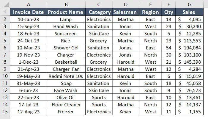
The dataset contains sales reports of different products. Additionally, it also includes category, salesman, region, quantity, and date. Now, I will create 2 Pivot Tables and connect two slicers in Excel.

Step 1: Create a Pivot Table in Excel

To create a Pivot Table in Excel, follow the steps below:

1. Select the entire range.
2. Go to the Insert tab > PivotTable dropdown > From Table/Range option.
   
3. Confirm the range and choose the location to place the Pivot Table.
4. Click OK.
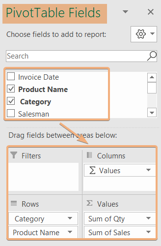
5. Drag the fields to areas from the PivotTable Fields.
6. Repeat the same steps to insert another Pivot Table.
   

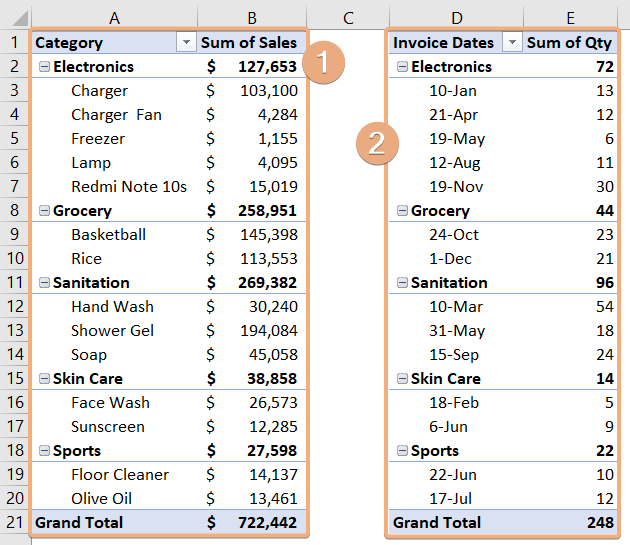
Here, I have inserted two Pivot Tables in Excel. In the Pivot Table 1, I have inserted category and product names in Rows and sales in the Columns area. Next, I inserted the category and invoice date in Rows and quantity in the Columns area.

Step 2: Insert Slicers into the Pivot Table

Now, I will put two slicers in the Pivot Table. So, I’m going to add the salesman and region fields to the two slicers. To do that, go through the steps below:

1. Select any cell in the Pivot Table.
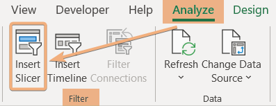
2. Go to the Analyze tab in the PivotTable Tools.
3. Click on the Insert Slicer under the Filter group.
   
4. In the Insert Slicers dialog box, check on the fields and click OK.
   

This will insert the selected slicers in the Excel Pivot Table. For Pivot Table 1, I have selected the salesman field and for Pivot Table 2, it is region.

Step 3: Connect the Slicers in Excel Pivot Table

Now, I will connect these two slicers in this Excel Pivot Table. So, have the guidelines below:

1. Select any of the slicers.
2. Right-click on that.
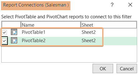
3. Click on Report Connections.
4. In the Report Connections dialog box, check on both Pivot Tables in Excel.
5. Click OK.
   
6. Do the same for other slicers in the Pivot Table.

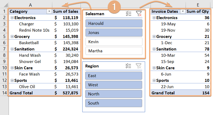
Now, if you filter on any of the slicers, you can filter both the Pivot Table in Excel. This image shows the filtered Pivot Table with slicer 1.
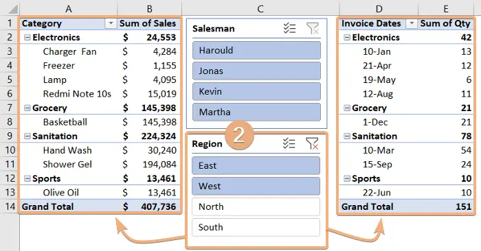
Now, this picture shows the filtered Pivot Table with slicer 2.

Conclusion

In conclusion, connecting two slicers in Excel can significantly enhance the flexibility and interactivity of your data analysis. By linking slicers, you create a seamless and dynamic experience that allows users to explore multiple dimensions of the data simultaneously. In the article, I have provided a step-by-step guide to connect two slicers in Excel Pivot Table.

Frequently Asked Questions

How do I connect one slicer to another slicer?

To connect one slicer to another in Excel:

1. Go to the Insert tab, click Slicer, and choose the field you want to filter.
2. Repeat the process to create a second slicer for another field.
3. Right-click on the first slicer and choose Report Connections.
4. In the Report Connections dialog box, select the checkbox corresponding to the sheet or PivotTable containing the second slicer. Click OK to establish the connection.

Now, when you use the first slicer to filter data, the second slicer will automatically adjust based on your selection. By following these steps, you can easily connect one slicer to another in Excel, creating a dynamic relationship between the slicers for synchronized data filtering.

Is there a way to combine slicers in Excel?

Excel doesn’t have a built-in feature to combine or merge slicers directly. Each slicer is typically associated with a specific PivotTable or PivotChart. However, you can achieve a similar effect by placing multiple slicers close together and configuring them to filter the same Pivot Table or Pivot Chart. This way, users can make selections from any of the slicers to apply combined filtering.

Here are steps to simulate combining slicers in Excel:

1. Generate slicers for the same field in different Pivot Tables or Pivot Charts.
2. Arrange the slicers near each other on the worksheet.
3. Right-click on each slicer, go to Slicer Settings and confirm that they are filtering the same data field.
4. Users can now make selections from any of the slicers, and the combined effect will be reflected in the associated Pivot Table or Pivot Chart.

While this method doesn’t physically combine slicers, it achieves a similar outcome by allowing users to interact with multiple slicers that affect the same data. Remember that features in Excel may evolve, so it’s advisable to check the latest Excel documentation for any updates or new features related to slicers.

How do you sync slicers in Excel?

To sync slicers in Excel, go through the steps below:

1. Generate slicers for the desired fields in different Pivot Tables or Pivot Charts.
2. Click on a slicer to select it.
3. Right-click on the selected slicer, then choose Report Connections.
4. In the Report Connections dialog, select the checkboxes corresponding to the Pivot Tables or Pivot Charts you want to sync with the slicer.
5. Click OK to confirm and establish the connection.

Now, when you use the slicer to filter data in one Pivot Table or Pivot Chart, all other connected Pivot Tables or Pivot Charts will automatically reflect the same filter criteria. This synchronization ensures consistency across multiple components of your Excel workbook.

Can you group a slicer?

Excel doesn’t provide a built-in feature to directly group slicers. Slicers are generally designed to work independently for individual Pivot Tables or Pivot Charts.

However, you can simulate a grouping effect by placing multiple slicers close together and configuring them to filter the same data field. This allows users to make selections from any of the slicers to apply combined filtering. Here are simplified steps:
Create multiple slicers for the same field in different Pivot Tables or Pivot Charts.

1. Position the slicers near each other on the worksheet.
2. Right-click on each slicer, go to Slicer Settings and confirm they are filtering the same data field.
3. Users can now make selections from any slicer, and the combined effect will be reflected in associated Pivot Tables or Pivot Charts.

While this method doesn’t group slicers in a formal sense, it achieves a similar outcome by allowing users to interact with multiple slicers that affect the same data. It’s important to check the latest Excel documentation for any updates or new features related to slicers, as Excel features may evolve.

How do I link slicers to a pivot chart?

To link slicers to a Pivot Chart in Excel:

1. Create Slicer: Insert a slicer for the desired field by going to the Insert tab, clicking Slicer, and choosing the relevant field.
2. Select PivotChart: Click on the Pivot Chart that you want to connect the slicer to.
3. Go to PivotChart Analyze Tab: Navigate to the Analyze tab on the Excel ribbon.
4. Insert Slicer: In the Filter group, click Insert Slicer and choose the slicer you created earlier.
5. Position Slicer: Arrange the slicer near the Pivot Chart for easy user access.

Now, when users interact with the slicer, the Pivot Chart will dynamically update based on the selected slicer values. This linkage enhances interactivity and enables users to easily filter and analyze data in the associated Pivot Chart.